Appendix S Mass Conservation Model
S.1 Intent
The TUFLOW FV Water Quality (WQ) Module is supported by a downloadable model suite that is intended to provide users with simple three dimensional models that can be used to:
- Assess WQ Module mass conservation performance, and/or
- Support exploration of the features and behaviour of the WQ Module, and/or
- Use as templates for building water quality control files for other simulations
The suite does not need a licence to execute with either existing or altered water quality parameters.
This Appendix provides background, analysis and windows usage instructions for the mass conservation model. The model suite can be run on either windows or linux, however this document describes only the windows execution process. TUFLOW FV releases from 2022 onward include the WQ Module and therefore can execute this model.
S.2 Description
The mass conservation model is configured as follows.
- General
- 1 month (745 hours) duration
- Includes salinity, temperature (and heat calculations), sediment and varying numbers of water quality computed variables
- 15 minute output
- 15 minute water quality simulation timestep
- Designed to mimic a deep lake that cools over an autumnal period
- Geometry
- Four three-dimensional flat bottomed columns, with the same bed elevation
- Lateral cell areas each of approximately 10 km\(^2\)
- Depth of 21 metres
- 20 vertical layers of variable thickness, with 17 fixed and 3 sigma (which span the top portion of the water column)
- Boundary conditions
- No inflows, outflows or other flow boundaries
- Meteorological boundaries applied
- Hourly timestep, 15 minute update
- Typical mid latitude autumnal conditions, with rainfall included
- Water quality parameterisation
- WQ Module control files that present the parameters used are included below for each simulation
- Each simulation includes the most complex simulation construction (for each simulation class) so as to stress test all available processes
- Parameters are set to be generally within expected ranges, with some deliberate exceptions designed to illustrate the parameter checking features of the WQ Module
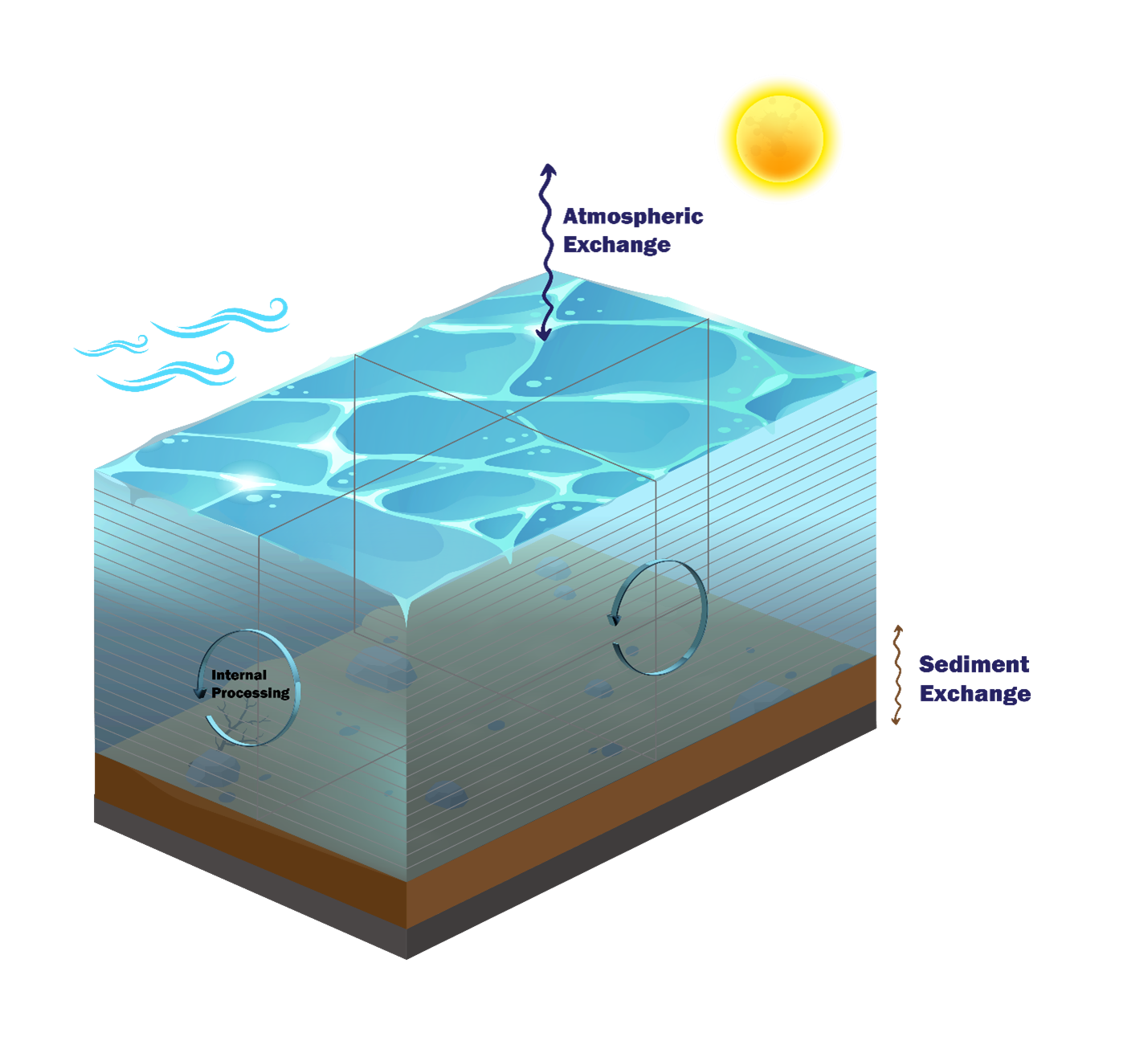
Figure S.1: WQ Module Mass Conservation Model
This setup of essentially stationary water is designed to be challenging for mass conservation. In particular, the exclusion of external flow boundaries (that can reset or overwhelm internal process calculations) is deliberate. These conditions might mimic a low rainfall lacustrine environment.
S.3 Model suite
The mass conservation model suite comprises six (6) related models. These six models are split into two groups of three, with these groups being identical other than one group using the milligrams per litre (MGL) units system and the other group using the millimoles per cubic metre (MMM) units system.
The three models within each group increase in configurational complexity that matches the three currently available water quality simulation classes. These are (with links to the relevant manual sections):
- Water quality simulation class == DO (Section 3.1)
- Water quality simulation class == inorganics (Section 3.2)
- Water quality simulation class == organics (Section 3.3)
Detailed model access and execution instructions are provided in Section S.6.
S.4 Calculations
The primary calculation used to assess mass conservation for each computed variable \(X\) follows:
\[\begin{equation} X_{mb}(t) = 100 \times \frac{X_{mp}(t) - X_{mi}(t)}{X_{mi}(t)} \tag{S.1} \end{equation}\] where \(X_{mb}(t)\) is the percentage difference between two methods of computing the mass of computed variable \(X\) in the domain:
- \(X_{mp}(t)\): Progressively modifying the initial domain mass by adding to it the sum of the relevant fluxes \(F_i\) at each timestep \(t\). No resetting of this calculation occurs - it is designed (stringently) such that any mass conservation errors will accumulate in time
- \(X_{mi}(t)\): Multiplying the reported concentrations of \(X\) in cell \(j\) of volume \(V_j\) and integrating over the entire model domain at each timestep \(t\). This mass is reset at each timestep and corresponds to the mass reported by TUFLOW FV
\(X_{mp}(t)\) and \(X_{mi}(t)\) are computed as per Equation (S.2). \(F_{i}(t)\) are the relevant fluxes for \(X\) (up to a total number of \(i=NF\) fluxes) and are converted from per area (or per volume) and per time amounts to mass amounts. The number of cells in the domain is \(NC\), and \(\left[X\right]_{j}(t)\) is the concentration of computed variable \(X\) in cell \(j\) at time \(t\). The model contains sigma layers and as such \(V_{j}\) may be time varying.
\[\begin{equation} \left.\begin{aligned} X_{mp}(t) =& \sum_{j=1}^{NC} \left[X\right]_{j}(0) \times V_j(0) + \sum_{i=1}^{NF} F_{i}(t) \\ \\ X_{mi}(t) =& \sum_{j=1}^{NC} \left[X\right]_{j}(t) \times V_j(t) \end{aligned}\right\} \tag{S.2} \end{equation}\]
As a general note, reported fluxes need to be used with care in mass conservation analyses. This is because fluxes are reported as instantaneous values, and are not integrated or accumulated between overall model output file writing timesteps. For example, if water quality calculations are undertaken every 15 minutes but outputs are written every hour, then several water quality calculations are undertaken between reporting. Whilst the hourly output water quality concentrations will correctly reflect the action of fluxes at every 15 minute increment, the output fluxes will be instantaneous, and equal to those that happen to be occurring at the hourly output time. They will not necessarily be reflective of the fluxes that occurred over the course of the preceding hour. Using these fluxes in mass conservation calculations can therefore lead to spurious outcomes. One solution to this matter is to set the output and water quality (and boundary condition update) timesteps to be the same in mass conservation analyses, noting that this may however generate large output files.
Three simulations were executed, with one for each of the DO, inorganics and organics simulation classes. The timeseries of \(X_{mb}(t)\), together with the fluxes used in calculations, are presented below for all relevant computed variables. The WQ Module control file commands are also included for reference. Only the MGL units system predictions and calculations are presented.
S.5 Mass conservation performance
S.5.1 Simulation class: DO
This is the simplest simulation class and it has oxygen as the only mandatory model class. For illustrative purposes, the optional pathogens model class has also been included in this mass balance simulation. The computed variables presented are therefore:
- Dissolved oxygen
- Pathogen 1 (which includes attachment dynamics)
- Pathogen 2 (which excludes attachment dynamics)
The initial conditions are:
- Dissolved oxygen: 8.0 mg/L
- Pathogen 1 alive, attached and dead: 1e6 CFU/100mL, 1e5 CFU/100mL, 1e5 CFU/100mL
- Pathogen 2 alive and dead: 1e5 CFU/100mL, 1e4 CFU/100mL
The relevant fluxes considered are (coloured as
- Dissolved oxygen
Sediment - Atmospheric (both source and sink)
- Pathogen 1
Natural mortality Inactivation due to irradiance - Attachment and detachment
Settling
- Pathogen 2
Natural mortality Inactivation due to irradiance Settling
The mass conservation performance of the WQ Module for dissolved oxygen and summed pathogens (i.e. pathogen 1 and pathogen 2 combined) is presented in Figure S.2, via \(DO_{mb}\), \(PTHa_{mb}\) and \(PTHd_{mb}\). Over the duration of the simulation, mass conservation holds to within 0.02%. It is noted that the alive pathogens mass balance (\(PTHa_{mb}\)) is truncated at 2 weeks because alive concentrations are six orders of magnitude lower that initial conditions by this time, and this pushes mass balance percentage error calculations to approach a divide by zero. Dead pathogen mass conservation is less affected because overall changes are approximately one order of magnitude only. Relevant fluxes used to compute this mass conservation, as well as total pathogen mass conservation, are presented subsequently.
Figure S.2: Dissolved oxygen mass conservation parameters \(DO_{mb}(t)\), \(PTHa_{mb}(t)\) and \(PTHd_{mb}(t)\)
Figure S.3: Dissolved oxygen WQ Module fluxes \(F_i(t)\) used to compute \(DO_{mp}(t)\)
The following are pathogen fluxes. Because fluxes vary by several orders of magnitude, they are presented as logarithms, as -log\(_{10}\)(-flux). For example, a plotted value of -15 below, means that the actual flux was -1e15 CFU/15 minutes (not 1e-15 CFU/15 minutes), and a change in value from -16 to -15 represents a tenfold decrease in flux.
Figure S.4: Pathogen WQ Module fluxes \(F_i(t)\) used to compute \(PTHa_{mp}(t)\) and \(PTHd_{mp}(t)\)
Figure S.5: Total pathogen mass conservation parameter \(PTHT_{mb}(t)\)
Following are the WQ Module control file commands used to generate the above.
simulation class == DO
wq dt == 900.0
wq units == mgl
oxygen model == O2
oxygen min max == 0.0, 12.0
oxygen benthic == 4.7, 1.08
end oxygen model
pathogen model == attached, pth1
alive min max == 0.0, 1e7
mortality == 0.0008, 0.0, 6.1, 1.0, 1.14
visible inactivation == 0.0, 0.0667, 0.1
uva inactivation == 0.01, 0.00667, 0.1
uvb inactivation == 0.02, 0.00667, 0.1
settling == -0.001, -0.2
target attached fraction == 0.5
end pathogen model
pathogen model == free, pth2
alive min max == 0.0, 1e7
mortality == 0.08, 2e-12, 6.1, 1.0, 1.11
visible inactivation == 0.082, 0.0067, 0.5
uva inactivation == 0.5, 0.0067, 0.5
uvb inactivation == 1.0, 0.0067, 0.5
settling == -0.03
end pathogen model
material == default
oxygen flux == -1400.0
end material
material == 1
oxygen flux == -1100.0
end material
material == 2
oxygen flux == -1200.0
end material
material == 3
oxygen flux == -1300.0
end material
S.5.2 Simulation class: Inorganics
The computed variables presented are:
- Dissolved oxygen
- Silicate
- Ammonium
- Nitrate
- FRP
- Adsorbed FRP
- Two phytoplankton groups (one each for the basic and advanced model)
Pathogen behaviour is unchanged from the DO simulation class mass balance model presented in Section S.5.1 so the corresponding mass balance is omitted for clarity.
The initial conditions are:
- Dissolved oxygen: 8.0 mg/L
- Silicate: 50.0 mg/L
- Ammonium: 0.15 mg/L
- Nitrate: 0.2 mg/L
- FRP: 0.04 mg/L
- Adsorbed FRP: 0.02 mg/L
- Blue green phytoplankton: 2.0 \(\mu\)g/L (advanced model)
- Blue green internal nitrogen: 0.008 mg/L
- Blue green internal phosphorus: 0.0012 mg/L
- Green phytoplankton: 5.0 \(\mu\)g/L (basic model)
The relevant fluxes considered are:
- Dissolved oxygen
Sediment - Atmospheric (both source and sink)
Nitrification Phytoplankton primary productivity Phytoplankton respiration
- Silicate
Sediment Phytoplankton primary productivity Phytoplankton mortality Phytoplankton excretion
- Ammonium
Sediment Atmospheric (wet and dry deposition) Nitrification Anaerobic oxidation of ammonium Dissimilatory reduction of nitrate to ammonium Phytoplankton primary productivity Phytoplankton mortality Phytoplankton excretion
- Nitrate
Sediment Atmospheric (wet and dry deposition)Nitrification Denitrification Anaerobic oxidation of ammonium Dissimilatory reduction of nitrate to ammonium Phytoplankton primary productivity
- FRP
Sediment Atmospheric Adsorption anddesorption Phytoplankton primary productivity Phytoplankton mortality Phytoplankton excretion
- FRP Adsorbed
Adsorption anddesorption
- Phytoplankton (both groups)
Phytoplankton primary productivity Phytoplankton respiration Phytoplankton mortality Phytoplankton excretion Phytoplankton sedimentation
The mass conservation performance of the WQ Module is presented in Figure S.6, via \(DO_{mb}(t)\), \(Si_{mb}(t)\), \(Amm_{mb}(t)\), \(Nit_{mb}(t)\), \((FRP+FRPAds)_{mb}(t)\) and \(PHY_{mb}(t)\). Over the duration of the simulation, mass conservation holds to within approximately 0.014%. Relevant fluxes used to compute these mass conservations, as well as total nitrogen and total phosphorus mass conservations, are presented subsequently.
Figure S.6: Inorganics mass conservation parameters \(DO_{mb}(t)\), \(Si_{mb}(t)\), \(Amm_{mb}(t)\), \(Nit_{mb}(t)\), \(FRP_{mb}(t)\) and \(PHY_{mb}(t)\)
Figure S.7: Dissolved oxygen WQ Module fluxes \(F_i(t)\) used to compute \(DO_{mb}(t)\)
Figure S.8: Silicate WQ Module fluxes \(F_i(t)\) used to compute \(Si_{mb}(t)\)
Figure S.9: Ammonium WQ Module fluxes \(F_i(t)\) used to compute \(Amm_{mb}(t)\)
Ammonium anammox fluxes are zero in the dissolved oxygen conditions of this mass conservation model.
Figure S.10: Nitrate WQ Module fluxes \(F_i(t)\) used to compute \(Nit_{mb}(t)\)
Nitrate anammox fluxes are zero in the dissolved oxygen conditions of this mass conservation model.
Figure S.11: FRP + FRPAds WQ Module fluxes \(F_i(t)\) used to compute \((FRP+FRPAds)_{mb}(t)\)
Figure S.12: Phytoplankton WQ Module fluxes \(F_i(t)\) used to compute \(PHY_{mb}(t)\)
Figure S.13: Inorganics total nitrogen and total phosphorus mass conservation parameters \(TN_{mb}(t)\) and \(TP_{mb}(t)\)
Following are the WQ Module control file commands used to generate the above.
simulation class == inorganics
wq dt == 900.0
wq units == mgl
oxygen model == O2
oxygen min max == 0.0, 12.0
oxygen benthic == 4.7, 1.08
end oxygen model
silicate model == si
silicate min max == 0.0, 100.0
silicate benthic == 4.2, 1.01
oxygen == on
end silicate model
inorganic nitrogen model == ammoniumnitrate
ammonium min max == 0.0, 50.0
nitrate min max == 0.0, 50.0
ammonium benthic == 4.05, 1.06
nitrate benthic == 4.25, 1.10
nitrification == 0.05, 4.15, 1.01
denitrification == michaelis menten, 0.05, 4.01, 1.03
oxygen == on
atmospheric deposition == 5.0, 0.0, 0.5
anaerobic oxidation of ammonium == 0.005, 2.5, 2.5
diss nitrate reduction to ammonium == 0.005, 5.0
end inorganic nitrogen model
inorganic phosphorus model == frphsads
FRP min max == 0.0, 5.0
FRP ads min max == 0.0, 5.0
FRP benthic == 4.3, 1.095
oxygen == on
atmospheric deposition == 0.5, 0.0
adsorption == linear, 0.25
settling == 0.000
end inorganic phosphorus model
phyto model == advanced, bluegreen
min max == 0.05, 50.0
temperature limitation == standard, 19.0, 22.0, 29.0
salinity limitation == mixed, 5.0, 10.0, 2.5
light limitation == chalker, 0.0005, 150.0
nitrogen limitation == 0.005, 1.5, 3.0, 5.0
phosphorus limitation == 0.002, 0.12, 0.3, 0.6
silicate limitation == 0.005, 9.0
uptake == 2.5, 0.3, 8.0
primary productivity == 3.4, 1.08
respiration == 0.06, 1.04, 0.2, 0.3, 0.1
carbon chla ratio == 26.8
nitrogen fixing == 0.002, 0.3
settling == constant, -0.3
end phyto model
phyto model == basic, green
min max == 0.05, 50.0
temperature limitation == standard, 19.0, 22.0, 29.0
salinity limitation == fresh, 2.0, 5.0, 0.0
light limitation == steele, 0.0005, 150.0
nitrogen limitation == 0.01, 2.5
phosphorus limitation == 0.005, 0.05
silicate limitation == 0.01, 4.0
uptake == 3.0, 0.6, 8.0
primary productivity == 2.6, 1.1
respiration == 0.005, 1.1, 0.3, 0.4, 0.5
carbon chla ratio == 27.8
nitrogen fixing == 0.001, 0.5
settling == constant, -0.4
end phyto model
pathogen model == attached, pth1
alive min max == 0.0, 1e7
mortality == 0.0008, 0.0, 6.1, 1.0, 1.14
visible inactivation == 0.0, 0.0667, 0.1
uva inactivation == 0.01, 0.00667, 0.1
uvb inactivation == 0.02, 0.00667, 0.1
settling == -0.001, -0.2
target attached fraction == 0.5
end pathogen model
pathogen model == free, pth2
alive min max == 0.0, 1e7
mortality == 0.08, 2e-12, 6.1, 1.0, 1.11
visible inactivation == 0.082, 0.0067, 0.5
uva inactivation == 0.5, 0.0067, 0.5
uvb inactivation == 1.0, 0.0067, 0.5
settling == -0.03
end pathogen model
material == default
oxygen flux == -1400.0
silicate flux == 10.0
ammonium flux == 20.0
nitrate flux == 30.0
frp flux == 5.0
end material
material == 1
oxygen flux == -1100.0
silicate flux == 11.0
ammonium flux == 21.0
nitrate flux == 31.0
frp flux == 6.0
end material
material == 2
oxygen flux == -1200.0
silicate flux == 12.0
ammonium flux == 22.0
nitrate flux == 32.0
frp flux == 7.0
end material
material == 3
oxygen flux == -1300.0
silicate flux == 13.0
ammonium flux == 23.0
nitrate flux == 33.0
frp flux == 8.0
end materialS.5.3 Simulation class: Organics
The computed variables presented are:
- Dissolved oxygen
- Silicate
- Ammonium
- Nitrate
- FRP
- Adsorbed FRP
- Particulate organic carbon
- Dissolved organic carbon
- Particulate organic nitrogen
- Dissolved organic nitrogen
- Particulate organic phosphorus
- Dissolved organic phosphorus
- Refractory particulate organic matter
- Refractory dissolved organic carbon
- Refractory dissolved organic nitrogen
- Refractory dissolved organic phosphorus
- Two phytoplankton groups (one each for the basic and advanced model)
Again, pathogen behaviour is unchanged from the DO simulation class mass balance model presented in Section S.5.1 so the corresponding mass balance is omitted for clarity.
The initial conditions are:
- Dissolved oxygen: 8.0 mg/L
- Silicate: 1.0 mg/L
- Ammonium: 0.15 mg/L
- Nitrate: 0.2 mg/L
- FRP: 0.04 mg/L
- Adsorbed FRP: 0.02 mg/L
- Particulate organic carbon: 2.5 mg/L
- Dissolved organic carbon: 1.5 mg/L
- Particulate organic nitrogen: 0.3 mg/L
- Dissolved organic nitrogen: 0.1 mg/L
- Particulate organic phosphorus: 0.06 mg/L
- Dissolved organic phosphorus: 0.03 mg/L
- Refractory particulate organic matter: 2.1 mg/L
- Refractory dissolved organic carbon: 1.6 mg/L
- Refractory dissolved organic nitrogen: 0.6 mg/L
- Refractory dissolved organic phosphorus: 0.04 mg/L
- Blue green phytoplankton: 2.0 \(\mu\)g/L (advanced model)
- Blue green internal nitrogen: 0.008 mg/L
- Blue green internal phosphorus: 0.0012 mg/L
- Green phytoplankton: 5.0 \(\mu\)g/L (basic model)
The relevant fluxes considered are:
- Dissolved oxygen
Sediment - Atmospheric (both source and sink)
Nitrification Dissolved organic carbon mineralisation (oxygen based) Phytoplankton primary productivity Phytoplankton respiration
- Silicate
Sediment Phytoplankton primary productivity Phytoplankton mortality Phytoplankton excretion
- Ammonium
Sediment Atmospheric (wet and dry deposition) Nitrification Anaerobic oxidation of ammonium Dissimilatory reduction of nitrate to ammonium Dissolved organic nitrogen mineralisation Dissolved refractory organic matter photolysis Phytoplankton primary productivity
- Nitrate
Sediment Atmospheric (wet and dry deposition) Nitrification Denitrification Anaerobic oxidation of ammonium Dissimilatory reduction of nitrate to ammonium Dissolved organic carbon mineralisation (nitrate based) Phytoplankton primary productivity flux
- FRP
Sediment Atmospheric Adsorption anddesorption Dissolved organic phosphorus mineralisation Dissolved refractory organic matter photolysis Phytoplankton primary productivity
- FRP Adsorbed
Adsorption anddesorption
- Particulate organic carbon, nitrogen and phosphorus
Hydrolysis Breakdown of refractory particulate organic matter Phytoplankton mortality
- Dissolved organic carbon, nitrogen and phosphorus
Sediment Hydrolysis Mineralisation Dissolved refractory organic matter photolysis Dissolved refractory organic matter activation Phytoplankton excretion
- Refractory particulate organic matter
Breakdown
- Refractory organic carbon, nitrogen and phosphorus
Dissolved refractory organic matter photolysis Dissolved refractory organic matter activation
- Phytoplankton (both groups)
Phytoplankton primary productivity Phytoplankton respiration Phytoplankton mortality Phytoplankton excretion Phytoplankton sedimentation
The mass conservation performance of the WQ Module is presented in Figure S.14, via \(DO_{mb}(t)\), \(Si_{mb}(t)\), \(Amm_{mb}(t)\), \(Nit_{mb}(t)\), \((FRP+FRPAds)_{mb}(t)\), \(POC_{mb}(t)\), \(DOC_{mb}(t)\), \(PON_{mb}(t)\), \(DON_{mb}(t)\), \(POP_{mb}(t)\), \(DOP_{mb}(t)\), \(RPOM_{mb}(t)\), \(RDOC_{mb}(t)\), \(RDON_{mb}(t)\), \(RDOP_{mb}(t)\) and \(PHY_{mb}(t)\). Over the duration of the simulation, mass conservation holds to within 0.024%. Relevant fluxes used to compute these mass conservations, as well as total nitrogen and total phosphorus mass conservations, are presented subsequently.
Figure S.14: Organics mass conservation parameters \(DO_{mb}(t)\), \(Si_{mb}(t)\), \(Amm_{mb}(t)\), \(Nit_{mb}(t)\), \(FRP_{mb}(t)\), \(POC_{mb}(t)\), \(DOC_{mb}(t)\), \(PON_{mb}(t)\), \(DON_{mb}(t)\), \(POP_{mb}(t)\), \(DOP_{mb}(t)\), \(RPOM_{mb}(t)\), \(RDOC_{mb}(t)\), \(RDON_{mb}(t)\), \(RDOP_{mb}(t)\) and \(PHY_{mb}(t)\)
Figure S.15: Dissolved oxygen WQ Module fluxes \(F_i(t)\) used to compute \(DO_{mb}(t)\)
Figure S.16: Silicate WQ Module fluxes \(F_i(t)\) used to compute \(Si_{mb}(t)\)
Figure S.17: Ammonium WQ Module fluxes \(F_i(t)\) used to compute \(Amm_{mb}(t)\)
Ammonium anammox fluxes are zero in the dissolved oxygen conditions of this mass conservation model.
Figure S.18: Nitrate WQ Module fluxes \(F_i(t)\) used to compute \(Nit_{mb}(t)\)
Nitrate anammox fluxes are zero in the dissolved oxygen conditions of this mass conservation model.
Figure S.19: FRP+FRPAds WQ Module fluxes \(F_i(t)\) used to compute \((FRP+FRPAds)_{mb}(t)\)
Figure S.20: POC WQ Module fluxes \(F_i(t)\) used to compute \(POC_{mb}(t)\)
Figure S.21: DOC WQ Module fluxes \(F_i(t)\) used to compute \(DOC_{mb}(t)\)
Figure S.22: PON WQ Module fluxes \(F_i(t)\) used to compute \(PON_{mb}(t)\)
Figure S.23: DON WQ Module fluxes \(F_i(t)\) used to compute \(DON_{mb}(t)\)
Figure S.24: POP WQ Module fluxes \(F_i(t)\) used to compute \(POP_{mb}(t)\)
Figure S.25: DOP WQ Module fluxes \(F_i(t)\) used to compute \(DOP_{mb}(t)\)
Figure S.26: RPOM WQ Module fluxes \(F_i(t)\) used to compute \(RPOM_{mb}(t)\)
Figure S.27: RDOC WQ Module fluxes \(F_i(t)\) used to compute \(RDOC_{mb}(t)\)
Figure S.28: RDON WQ Module fluxes \(F_i(t)\) used to compute \(RDON_{mb}(t)\)
Figure S.29: RDOP WQ Module fluxes \(F_i(t)\) used to compute \(RDOP_{mb}(t)\)
Figure S.30: Phytoplankton WQ Module fluxes \(F_i(t)\) used to compute \(PHY_{mb}(t)\)
Figure S.31: Organics total nitrogen and total phosphorus mass conservation parameters \(TN_{mb}(t)\) and \(TP_{mb}(t)\)
Following are the WQ Module control file commands used to generate the above.
simulation class == organics
wq dt == 900.0
wq units == mgl
oxygen model == O2
oxygen min max == 0.0, 12.0
oxygen benthic == 4.7, 1.08
end oxygen model
silicate model == si
silicate min max == 0.0, 100.0
silicate benthic == 4.2, 1.01
oxygen == on
end silicate model
inorganic nitrogen model == ammoniumnitrate
ammonium min max == 0.0, 50.0
nitrate min max == 0.0, 50.0
ammonium benthic == 4.05, 1.06
nitrate benthic == 4.25, 1.10
nitrification == 0.05, 4.15, 1.01
denitrification == michaelis menten, 0.05, 4.01, 1.03
oxygen == on
atmospheric deposition == 5.0, 0.0, 0.5
anaerobic oxidation of ammonium == 0.005, 2.5, 2.5
diss nitrate reduction to ammonium == 0.005, 5.0
end inorganic nitrogen model
inorganic phosphorus model == frphsads
FRP min max == 0.0, 5.0
FRP ads min max == 0.0, 5.0
FRP benthic == 4.3, 1.095
oxygen == on
atmospheric deposition == 0.5, 0.0
adsorption == linear, 0.25
settling == 0.000
end inorganic phosphorus model
phyto model == advanced, bluegreen
min max == 0.05, 50.0
temperature limitation == standard, 19.0, 22.0, 29.0
salinity limitation == mixed, 5.0, 10.0, 2.5
light limitation == chalker, 0.0005, 150.0
nitrogen limitation == 0.005, 1.5, 3.0, 5.0
phosphorus limitation == 0.002, 0.12, 0.3, 0.6
silicate limitation == 0.005, 9.0
uptake == 2.5, 0.3, 8.0
primary productivity == 3.4, 1.08
respiration == 0.06, 1.04, 0.2, 0.3, 0.1
carbon chla ratio == 26.8
nitrogen fixing == 0.002, 0.3
settling == constant, -0.3
end phyto model
phyto model == basic, green
min max == 0.05, 50.0
temperature limitation == standard, 19.0, 22.0, 29.0
salinity limitation == fresh, 2.0, 5.0, 0.0
light limitation == steele, 0.0005, 150.0
nitrogen limitation == 0.01, 2.5
phosphorus limitation == 0.005, 0.05
silicate limitation == 0.01, 4.0
uptake == 3.0, 0.6, 8.0
primary productivity == 2.6, 1.1
respiration == 0.005, 1.1, 0.3, 0.4, 0.5
carbon chla ratio == 27.8
nitrogen fixing == 0.001, 0.5
settling == constant, -0.4
end phyto model
organic matter model == refractory
carbon min max == 0.0, 10.0, 0.0, 10.0
nitrogen min max == 0.0, 10.0, 0.0, 10.0
phosphorus min max == 0.0, 9.0, 0.0, 9.0
organics benthic == 1.0, 1.08
hydrolysis == 0.05, 0.007, 0.0004, 1.0, 1.05
mineralisation == 0.01, 1.2, 1.03, 0.5, 0.5
self shading == 0.0, 0.0
settling == stokes, 0.00000035, 2450.8
ref carbon min max == 0.0, 10.0, 0.0, 10.0
ref nitrogen min max == 0.0, 10.0
ref phosphorus min max == 0.0, 9.0
ref breakdown == 0.001, 0.1, 0.01
ref activation == 0.01
ref photolysis == 0.5
ref self shading == 0.0, 0.0
ref settling == stokes, 0.00000045, 2450.8
end organic matter model
pathogen model == attached, pth1
alive min max == 0.0, 1e7
mortality == 0.0008, 0.0, 6.1, 1.0, 1.14
visible inactivation == 0.0, 0.0667, 0.1
uva inactivation == 0.01, 0.00667, 0.1
uvb inactivation == 0.02, 0.00667, 0.1
settling == -0.001, -0.2
target attached fraction == 0.5
end pathogen model
pathogen model == free, pth2
alive min max == 0.0, 1e7
mortality == 0.08, 2e-12, 6.1, 1.0, 1.11
visible inactivation == 0.082, 0.0067, 0.5
uva inactivation == 0.5, 0.0067, 0.5
uvb inactivation == 1.0, 0.0067, 0.5
settling == -0.03
end pathogen model
material == default
oxygen flux == -1400.0
silicate flux == 10.0
ammonium flux == 20.0
nitrate flux == 30.0
frp flux == 5.0
doc flux == 20.0
don flux == 10.0
dop flux == 5.0
end material
material == 1
oxygen flux == -1100.0
silicate flux == 11.0
ammonium flux == 21.0
nitrate flux == 31.0
frp flux == 6.0
doc flux == 19.0
don flux == 9.0
dop flux == 4.0
end material
material == 2
oxygen flux == -1200.0
silicate flux == 12.0
ammonium flux == 22.0
nitrate flux == 32.0
frp flux == 7.0
doc flux == 18.0
don flux == 8.0
dop flux == 3.0
end material
material == 3
oxygen flux == -1300.0
silicate flux == 13.0
ammonium flux == 23.0
nitrate flux == 33.0
frp flux == 8.0
doc flux == 17.0
don flux == 7.0
dop flux == 2.0
end materialS.6 Access and execution
S.6.1 Access
To download the mass conservation model:
- Download the zip from the TUFLOW website by clicking here (under Example / Demo Models section)
- Unzip the model in a convenient location. For the purposes of this description, the location of the mass conservation model suite is assumed to be:
- ‘C:\TUFLOWFV\Models\’
The above steps will create a subfolder called ‘wqm’ within the chosen folder location. Within this wqm subfolder will be another subfolder called mass_conservation_model. This is where the mass conservation model resides.
S.6.2 Execution
Unzipping the above will generate the folder structure within C:\TUFLOWFV\Models\wqm\mass_conservation_model\ as below.
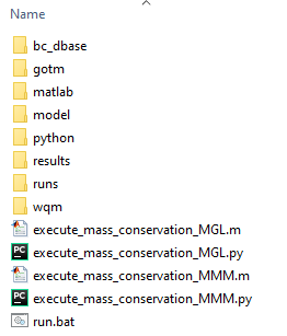
Figure S.32: Mass conservation model folder structure
The above C:\TUFLOWFV\Models\wqm\mass_conservation_model\ subfolders are as follows:
- bc_dbase: Boundary condition data
- gotm: External turbulence model namelist file
- matlab: MATLAB post processing files for mass conservation analysis
- model: Model geometry and related data
- python: Python post processing files for mass conservation analysis
- results: Model results (will be empty on initial download)
- runs: TUFLOW FV hydrodynamic and sediment transport control files
- wqm: TUFLOW FV WQ Module control files
The C:\TUFLOWFV\Models\wqm\mass_conservation_model\ folder should also contain five files:
- execute_mass_conservation_MGL.m: Executes mass conservation calculations in MATLAB for MGL simulations
- execute_mass_conservation_MGL.py: Executes mass conservation calculations in Python for MGL simulations
- execute_mass_conservation_MMM.m: Executes mass conservation calculations in MATLAB for MMM simulations
- execute_mass_conservation_MMM.py: Executes mass conservation calculations in Python for MMM simulations
- run.bat: Executes a mass conservation simulation
The mass conservation model can now be executed via a windows command line as follows:
- Open a windows command console
- Click the windows icon in the Task Bar once, and type ‘cmd’ (without the apostrophes) and then hit enter. A command console will appear, with the prompt being in a default directory.
- Navigate to the directory in which the mass conservation model resides by typing the following (noting that these instructions use the assumed folder location above)
cd C:\TUFLOWFV\Models\wqm\mass_conservation_model\
- Type the following, with user specified arguments being bracketed as <argument> and are separated by a single space:
run <simulation class> <units system> <exe path>
Each of the arguments above have the following options:
- <simulation class>:
- DO
- inorganics
- organics
- <units system>:
- MGL
- MMM
- <exe path>:
- The full path to the TUFLOW FV executable, here assumed to be C:\TUFLOWFV\EXE\TUFLOWFV.EXE. If there are spaces in the path name to an executable, then enclose the argument in inverted commas, e.g. “C:\TUFLOW FV\EXE\TUFLOWFV.EXE”
Example commands using the above are therefore:
run DO MGL C:\TUFLOWFV\EXE\TUFLOWFV.EXE
This will execute the DO simulation class model in the milligrams per litre units system
run organics MMM C:\TUFLOWFV\EXE\TUFLOWFV.EXE
This will execute the organics simulation class model in the millimoles per cubic metre units system
S.7 Results
All relevant water quality and hydrodynamic computed variables and diagnostics are written to the output files produced by executing the above commands. In all cases, results are written to the results folder, and are named based on the executed simulation in the form:
- MB_<simulation class>_<units system>_<suffix>.nc
The <bracketed> options include:
- <simulation class>:
- DO
- inorganics
- organics
- <units system>:
- MGL
- MMM
- <suffix>:
- WQ
Example results files produced are therefore:
- MB_DO_MGL_WQ.nc
- This is the results file from a DO simulation class model in the milligrams per litre units system
- MB_INORGANICS_MMM_WQ.nc
- This is the results file from an inorganics simulation class model in the millimoles per cubic metre units system
Predictions of computed and diagnostic variables can be viewed and interrogated either:
- In QGIS in the same manner as any other TUFLOW FV results, following these instructions, and/or
- Using MATLAB and/or python tools
A log file reporting WQ Module simulation commentary is produced for every execution. This resides in the same folder as the WQ Module control file, and has the same name but with the file extension “fvwqlog”. The log file produced by the mass conservation model should be reviewed to support understanding of the model parameterisation and execution.
S.8 Mass conservation analysis
Two options are available to assess the mass conservation performance of the WQ Module. These use:
- MATLAB, or
- Python
These perform identical calculations but are offered to support users in their preference for post processing platforms. Both platforms can handle simulations that have used either the MGL or MMM units systems.
The mass conservation analysis (by its nature) deals with mass, and as such, whilst the MMM analysis expects millimoles inputs for both user parameters and WQ Module results files, the core of the analysis engine operates in units of mass. Mass conservation outcomes from both MGL and MMM units systems are similarly reported as mass (not moles) errors.
S.8.1 MATLAB
The MATLAB mass conservation scripts should be executed using MATLAB R2022a, or later.
S.8.1.1 Set up
The following steps set up the mass conservation analysis in MATLAB:
- Open a MATLAB session
- Navigate to the directory where the mass conservation model has been downloaded (assumed to be C:\TUFLOWFV\Models\wqm\mass_conservation_model\ here)
- Set the working directory to be the same location
- In the MATLAB editor (or any text editor), open either of the following mfiles, depending on the units systems being used (MGL or MMM):
- C:\TUFLOWFV\Models\wqm\mass_conservation_model\execute_mass_conservation_MGL.m, or
- C:\TUFLOWFV\Models\wqm\mass_conservation_model\execute_mass_conservation_MMM.m
These files:
- Control the mass conservation analysis, and
- Contain the user specifiable and alterable parameters that are required by the mass conservation analysis
In addition to the above, two folders that contain MATLAB scripts need to be added to the MATLAB path, including adding all subfolders. The mass conservation analysis uses scripts in these folders. These folders are:
- The MATLAB scripts provided here. This folder is named TUFLOWFV_Matlab_Utilities_001
- The functions folder included in the zip download, which (using the assumed download location) is here:
- C:\TUFLOWFV\Models\wqm\mass_conservation_model\matlab\functions\
None of the scripts in either of these folders should be edited.
S.8.1.2 Execution
The following steps execute the mass conservation analysis in MATLAB:
- Set the
runIDvariable in execute_mass_conservation_MGL.m or execute_mass_conservation_MMM.m to be the simulation desired. Do this by uncommenting the required line. This runID will need to be that of a simulation that has already been executed (see Section S.6.2). The naming convention is the same as the commands used previously in the command window to execute a simulation:- MB_<simulation class>_<units system>
- Make sure that the series of parameters set in execute_mass_conservation_MGL.m (or execute_mass_conservation_MMM.m) coincide exactly with those used to execute the relevant water quality simulation. Any differences will adversely impact mass conservation calculations. To do so:
- Only alter execute_mass_conservation_MGL.m (or execute_mass_conservation_MMM.m). Do not alter any other mfiles
- Within this mfile, only alter parameters in the section titled ‘% User inputs’:
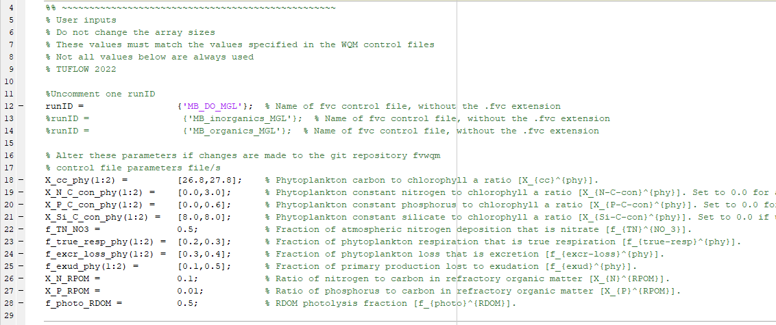
Figure S.33: Mass conservation mfile user inputs section
In this regard:
- Not all parameters are always used. For example, the DO simulation class uses none of the parameters listed in this section, other than runID
- Hyperlinks to the user manual descriptions of all parameters are included in the mfile
- Do not alter the lengths of the arrays – only change their values.
- Do not add further phytoplankton groups. The mass conservation model has two groups, with one each from the Basic and Advanced classes, so does not need additional groups to serve its purpose
- The user parameters must match those specified in the relevant WQ Module control file. If these differ then mass conservation will not hold. Ensure that any changes made to WQ Module control file parameters are mirrored in the parameter section shown above. The parameters in the WQ Module control files and MGL and MMM mfiles are consistent within the unchanged zip download
- Do not alter any other mfiles
To execute the mass conservation analysis, and having navigated to the MATLAB directory containing execute_mass_conservation_MGL.m (or execute_mass_conservation_MMM.m) type the following in the MATLAB command window:
execute_mass_conservation_MGL
for MGL units systems, or
execute_mass_conservation_MMM
for MMM units systems.
The following will initially appear (using the MB_DO_MGL model as an example)
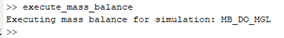
Figure S.34: Initial MATLAB commentary
If running the mass conservation process for the first time, a MATLAB warning similar to the following may appear. This can be ignored, and will not appear on subsequent runs of the same WQ Module simulation name:
- Could Not Find C:\TUFLOWFV\Models\wqm\mass_conservation_model\results\MB_DO_MGL_mass_conservation.xlsx
S.8.1.3 Outputs
All outputs are written to the results folder at:
- C:\TUFLOWFV\Models\wqm\mass_conservation_model\results\
Two results files are written (named according to simulation as above) in the units system adopted (MGL is used as an example here):
- MB_DO_MGL_mass_conservation.mat. This is a MATLAB datafile that contains all environment, flux and mass conservation data. The latter are timeseries, integrated over the entire mass conservation model domain. This can be loaded into MATLAB for further analysis using the MATLAB command (again, with varying name based on the runID):
load(‘C:\TUFLOWFV\Models\wqm\mass_conservation_model\results\MB_DO_MGL_mass_conservation.mat’)
- MB_DO_MGL_mass_conservation.xlsx. This contains the same flux and mass conservation data as MB_DO_MGL_mass_conservation.mat, but as columns in an Excel spreadsheet. These can also be used in further analysis as required
MATLAB also produces figures that graphically present the mass conservation analysis for every computed variable. The x- and y- axes are time (in hours) and mass conservation deviation (%), respectively. In the case of inorganics and organics simulation classes, an additional figure is produced that plots the same information, but for total nutrients. These figures can be reproduced using the data save in either MB_DO_MGL_mass_conservation.mat or MB_DO_MGL_mass_conservation.xlsx.
S.8.2 Python
The Python mass conservation scripts should be executed using Python 3.8, or later.
S.8.2.1 Set up
The following steps set up the mass conservation analysis in Python:
- Install Python (if not already installed). Python installation and configuration are required prior to executing the scripts provided. The steps to do so are presented here in the TUFLOW FV wiki.
- Install Python integrated development environment (IDE) (if not already installed). An IDE is used to control execution of the provided scripts. Any IDE can be used, although PyCharm is recommended and its setup is also described here in the TUFLOW FV wiki.
- Check that the following dependent Python packages are installed (e.g. using the command
pip listin the command line window if pip is installed), at the noted versions or later:- Numpy 1.19.0
- netCDF4 1.5.3
- pandas 1.2.4
- matplotlib 3.2.2
- openpyxl 3.0.10

Figure S.35: Check Python package versions in command prompt
- If any of these packages are missing then install package XXXX using the terminal command
pip install XXXXcommand. For example, if openpyxl is missing, then in the Python terminal typepip install openpyxl, and so on. - Open either of the following python script files in the Python IDE selected (PyCharm is recommended), depending on the units systems being used (MGL or MMM):
- C:\TUFLOWFV\Models\wqm\mass_conservation_model\execute_mass_conservation_MGL.py, or
- C:\TUFLOWFV\Models\wqm\mass_conservation_model\execute_mass_conservation_MMM.py
These files:
- Control the mass conservation analysis, and
- Contain the user specifiable and alterable parameters that are required by the mass conservation analysis
The python folder included in the zip download contains supplementary python scripts is here (using the assumed download location): - C:\TUFLOWFV\Models\wqm\mass_conservation_model\python\
Files in this folder should not be altered.
S.8.2.2 Execution
The following steps execute the mass conservation analysis in Python:
- Set the
runIDvariable in execute_mass_conservation_MGL.py or execute_mass_conservation_MMM.py to be the simulation desired. Do this by uncommenting the required line. This runID will need to be that of a simulation that has already been executed (see Section S.6.2). The naming convention is the same as the commands used previously in the command window to execute a simulation:- MB_<simulation class>_<units system>
- Make sure that the series of parameters set in execute_mass_conservation_MGL.py (or execute_mass_conservation_MMM.py) coincide exactly with those used to execute the relevant water quality simulation. Any differences will adversely impact mass conservation calculations. To do so:
- Only alter execute_mass_conservation_MGL.py (or execute_mass_conservation_MMM.py). Do not alter any other scripts
- Within this script, only alter parameters in the section titled ‘User inputs’. In this regard:
- Not all parameters are always used. For example, the DO simulation class uses none of the parameters listed in this section, other than runID
- Hyperlinks to the user manual descriptions of all parameters are included in the scripts.
- Do not alter the lengths of the arrays – only change their values.
- Do not add further phytoplankton groups. The mass conservation model has two groups, with one each from the Basic and Advanced classes, so does not need additional groups to serve its purpose
- The user parameters must match those specified in the relevant WQ Module control file. If these differ then mass conservation will not hold. Ensure that any changes made to WQ Module control file parameters are mirrored in the parameter section shown above. The parameters in the WQ Module control files and MGL and MMM scripts are consistent within the unchanged zip download
- Do not alter any other scripts
- Run the Python scripts execute_mass_balance_MGL.py or execute_mass_balance_MMM.py in the Python IDE. As an example, a script can be run by right-clicking its header and selecting ‘run’:
Figure S.36: Run scripts in PyCharm
The following warning messages can be ignored if they appear:
“MatplotlibDeprecationWarning: Adding an axes using the same arguments as a previous axes currently reuses the earlier instance. In a future version, a new instance will always be created and returned. Meanwhile, this warning can be suppressed, and the future behavior ensured, by passing a unique label to each axes instance.”
“No artists with labels found to put in legend. Note that artists whose label start with an underscore are ignored when legend() is called with no argument.”
A window will appear that displays the relevant plot. The figure window can be saved before closing by clicking on the save icon beneath the plot axes. The python script will exit once the plot window has been closed by the user. Some other messages may appear in the python console, but if the following message appears as the final run output, the script has run successfully.
Process finished with exit code 0
Following successful execution of the Python scripts, the outputs described in the next section will be generated.
S.8.2.3 Outputs
All outputs are written to the results folder at:
- C:\TUFLOWFV\Models\wqm\mass_conservation_model\results\
The result files are written (named according to simulation as above) in the units system adopted (MGL is used as an example here):
- MB_DO_MGL_mass_conservation.xlsx
This contains the flux and mass conservation data as columns in an Excel spreadsheet. These can also be used in further analysis as required.
The script also produces figures that graphically present the mass conservation analysis for every computed variable. The x- and y- axes are time (in hours) and mass conservation deviation (%), respectively. In the case of inorganics and organics simulation classes, an additional figure is produced that plots the same information, but for total nutrients. This additional figure is blank if a DO simulation is processed.
S.9 Notes
S.9.1 Units
The WQ Module offers simulation in one of two units systems: milligrams per litre (MGL) and millimoles per cubic metre (MMM). The mass conservation analysis provided with the WQ Module can therefore be run in both units systems. If users choose to do so, and then go on to compare mass conservation outcomes between the MGL and MMM units systems, some differences in behaviour may be observed. For instance, generally (but not always) the MMM system shows smaller cumulative mass conservation errors than its MGL parallel. The key reason for this is that the native computations units of the WQ Module are MMM, and as such, models set up in the MGL system have their MGL computed variable fields converted to and from MMM equivalents at each call by TUFLOW FV of the WQ Module (i.e. at every water quality timestep). These floating point arithmetic operations introduce very small (almost machine precision level) noise variations in computed variable fields that, given the accretive nature of mass conservation calculations, can accumulate over time. Conversely, these operations are bypassed if a user chooses to simulate in MMM units, and as such this noise is not incurred.
Notwithstanding the above, the deliberate design choices for the mass conservation model to be essentially static water and execute for a duration of one month (i.e. perform 2,976 water quality calls from TUFLOW FV), intentionally place great challenges on mass conservation. In this context, both the MGL and MMM units systems produce mass conservation errors less than 0.02% over the course of the simulation, which is entirely acceptable. This is orders of magnitude smaller than typical variations in environmental variables and indeed laboratory or field measurements against which model performance is often compared. The differences in mass conservation between the MGL and MMM units systems therefore reduce to being matters of academic computer science interest rather than of material concern to practitioners.
S.9.2 Precision
The mass conservation presented in this Appendix has used the single precision compilation of TUFLOW FV (noting that the WQ Module is always compiled in double precision). Testing of the same system has been undertaken using the corresponding double precision TUFLOW FV compilation. In general, the double precision mass conservation outcomes are better than single precision, as expected. As per Section S.9.1, however, these gains in conservation performance from single to double precision are immaterial to the practitioner who is concerned with the simulation of significantly less certain real world environmental systems and the verification of numerical model predictions to laboratory or field measurements.
S.9.3 Platform
The simulations and analyses presented in this section were undertaken using 64 bit windows binaries. Although not reported here, the mass conservation simulations were also all executed using linux binaries and the netcdf output files processed through the same scripts available in the zip download. Mass conservation results were unchanged.
