Section 4 Simulation Construction

4.1 Context

Previous sections have presented the architecture and water quality processes available within the WQ Module. This section describes the construction of a TUFLOW simulation with the WQ Module activated. This includes descriptions of all commands, with hyperlinks to the Appendices where commands and explanations are listed in a searchable and sortable table for ease of access. TUFLOW FV is the hydrodynamic model used in all descriptions that follow.

Optional model classes (such as pathogens) and their construction are first described in the simplest simulation class for which they can be deployed. Commentary on the ordering of optional constituents is provided in subsequent sections only where needed.

4.2 Units

The WQ Module allows for simulation construction in one of two unit systems (see Section 4.5.1):

A milligrams per litre system (which includes micrograms per litre for phytoplankton) that aligns with typical units of laboratory reporting, and
A millimoles per cubic metre system

A single units system must be adopted for a WQ Module simulation, and unit systems cannot be mixed within a simulation. This specification has implications for at least the setting of numerical values for:

Initial conditions
Boundary conditions
Computed variable parameters

When the milligrams per litre system is used, the WQ Module executes internal conversions between milligrams and millimoles, because millimoles are the units expected by the core water quality calculation routines. This conversion follows the form:

\[\begin{equation} n = \frac{m}{M} \tag{4.1} \end{equation}\] where $n$ is millimoles (mmol), $m$ is mass (mg) and $M$ is molar weight (mg/mmol). A similar concept applies to concentration and flux quantities. As such, the WQ Module assigns values to $M$ in converting from milligrams to millimoles, i.e. from user specified milligram initial conditions, boundary conditions and computed variable parameters, to the equivalent millimole quantities. The complete list of values of $M$ for all simulated constituents is provided in Table P.1. The two possibilities for units for each parameter are provided in Appendix R, where relevant.

As an example, if a user specifies the milligrams per litre units system (or allows the same default to be set) and sets FRP flux == 3.1 in a materials block, then this value of 3.1 is assumed to be mg/m$^2$/day. Consistent with typical laboratory reporting conventions (see below), this mass flux is taken to be that of elemental phosphorus $P$, not that of the phosphate molecule $PO_4^{3-}$. This would mean (using Table P.1 and Equation (4.1)) that the equivalent millimole rate would be computed as: \[\begin{equation} n = \frac{3.1}{31} = 0.1 \hspace{0.1cm} \text{mmol/m$^2$/day of P} \tag{4.2} \end{equation}\]

Given the above, users opting to construct WQ Module simulations in the milligrams units system need to clearly understand what is being reported in:

Field and/or laboratory measurements, and
Other numerical model predictions that may be used as WQ Module boundary conditions (such as catchment pollutant export models)

In the case of laboratory nutrient measurements, it is conventional to report concentrations of the typical quantities used by the WQ Module as silicate-Si, ammonium-N, nitrate-N, FRP-P, organic-C, organic-N, and organic-P. Whilst these quantities might be referred to informally as (for example) “nitrate concentrations”, the reported number is most commonly the concentration of elemental nitrogen contained within nitrate. To be clear, if a nitrate-N concentration is reported by a laboratory to be 3.5 mg/L, this means that in every litre of water, there are 3.5 milligrams of elemental nitrogen contained within nitrate molecules. Given the molar masses of elemental nitrogen and nitrate, this 3.5 milligrams of elemental N means that there are 15.5 milligrams of nitrate molecules (15.5 = 3.5 x 62/14) in the same litre of water. In this example, the concentration with which the WQ Module expects to be provided is 3.5 mg/L, not 15.5 mg/L.

The use of other model data to force WQ Module boundary conditions is also interpreted in this way. For example, a catchment model might report that an inflow to the WQ Module at an upstream riverine boundary condition has a “total nitrogen” concentration of 10.0 mg/L, and a user may have then speciated this to nitrate by applying a multiplicative factor of 0.15. If this resulting nitrate concentration of 1.5 mg/L is applied to the WQ Module as a boundary condition, it must be a concentration of elemental nitrogen within nitrate, which is consistent with what would be reported by a laboratory. This means that the user must be sure that the “total nitrogen” reported by the catchment model is in fact an elemental nitrogen concentration.

If users elect to construct WQ Module simulations in units of millimoles, then no internal WQ Module conversions take place, and the nature of the quantity (molecular or elemental) being specified is not relevant. For example, the user could specify millimoles units and a “FRP flux” of 0.1. This could be interpreted as a mmol/m$^2$/day rate of either the $PO_4^{3-}$ molecule, or just phosphorus $P$. This is because in one millimole of $PO_4^{3-}$, there is also one millimole of elemental $P$. The same one to one relationship holds for all other WQ Module relevant computed quantities (see Table P.1), other than oxygen which is treated as a diatomic molecule.

4.3 General arrangement

A water quality simulation is set up and executed under the umbrella of a TUFLOW FV control file (Figure 4.1, with other optional modules shown for illustrative purposes). That is:

The TUFLOW FV control file (*.fvc) file remains the central file that initiates and coordinates an overall simulation. This mirrors the way in which other TUFLOW FV modules, such as the ST Module and PT Module, are activated and executed
The TUFLOW FV control file contains a path to a separate WQ Module control file (*.fvwq) that in turn contains all the commands required to configure a WQ Module simulation

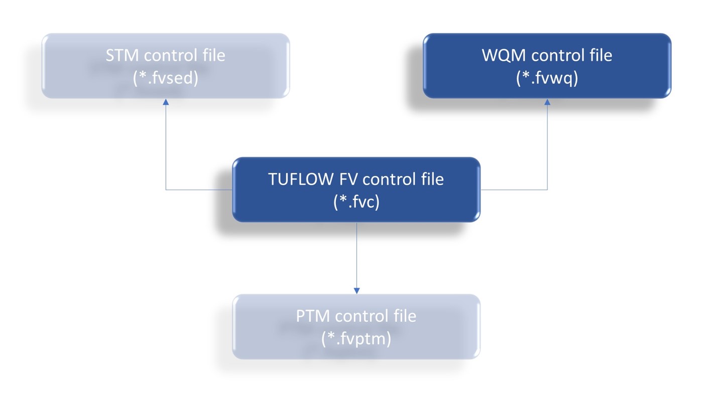
$\newcommand{\blockindent}{\hspace{0.5cm}}$

Figure 4.1: Simulation Coordination

TUFLOW FV and WQ Module control file commands are presented following.

4.4 TUFLOW FV control file commands

A TUFLOW FV simulation is executed as described in the TUFLOW FV user manual. If the WQ Module is to be activated in a simulation then the following commands are to be included.

4.4.1 WQ Module activation

Activation of the WQ Module is affected by specification of the following mandatory command in the TUFLOW control file:

water quality model == TUFLOW

Following this activation, TUFLOW FV will look for the specification of the name of the separate WQ Module control file via the following mandatory command:

water quality control file == <water quality control file name>.fvwq

This *.fvwq is separate to the *.fvc and contains user specified information that describes the configuration of the water quality simulation. If the *.fvwq is located in the same directory as the *.fvc, then this filename specification needs no associated path. It is recommended however that the *.fvwq be located in a directory separate to the *.fvc so that log and other related water quality specific files can be easily curated. If this approach is adopted, the following additional *.fvc command is required, noting that the folder path is specified as relative to the folder in which the *.fvc resides:

water quality model directory == <relative path to WQ directory>$\backslash$

This command must terminate in a $\backslash$ character. If this command is issued, then the *.fvwq water quality control file must be located in the directory specified.

In certain circumstances, executing water quality calculations in shallow cells can cause numerical instabilities. To control this behaviour, the WQ Module allows for water quality calculations to be switched off in cells that have depths less than a specified minimum (advection dispersion calculations will however continue to be performed - it is only the water quality-related non-conservative transformations that are turned off). This minimum depth (in meters) is specified in the TUFLOW FV *.fvc via the command:

cell water quality depth == $d_{min-wq}$

If this command is not issued then the default minimum depth of 0.01m (1cm) is applied.

This command parallels the TUFLOW FV command that controls the execution of hydrodynamic calculations as a function of water depth:

cell wet/dry depths == cell dry depth (m), cell wet depth (m)

In this TUFLOW FV command:

The cell dry depth value (default = 1.0e-06 m) corresponds to the water depth below which a cell is dropped completely from hydrodynamic (TUFLOW FV) computations (subject to the status of surrounding cells) and is therefore considered to be ‘dry’. Cells that have dried in a given time step are given a stat value of 0 in all TUFLOW FV results files, so this stat field acts as a mask to determine which cells are wet and dry when using post processing tools and or scripts. Dry cells are not contoured in QGIS or SMS when viewed, but appear as transparent. If set to a negative value the cell dry depth is set to zero.
The cell wet depth value (default = 1.0e-02 m) corresponds to the water depth below which a cell’s momentum is set to zero in order to avoid unphysical velocities at very low depths. The cell is not considered to be dry and therefore has a stat value of -1. If this value is less than or equal to the cell dry depth, it is set to the cell dry depth.

Given this, it is therefore recommended that across these commands and/or defaults, a user ensures that the following holds (as it does for the default values noted above):

\[\begin{equation} \text{cell dry depth} \lt \text{cell wet depth} \lt \text{cell water quality depth} \tag{4.3} \end{equation}\]

If, for example, cell water quality depth is set to a value less than cell dry depth, then water quality calculations will be attempted on cells that TUFLOW FV considers to be dry, which is to be avoided. If a situation arose where it was absolutely necessary, then cell water quality depth could be set to a value less than cell wet depth (but still greater than cell dry depth), but this is not recommended. To summarise, and if the recommended relative magnitudes of depths presented in Equation (4.3) is adopted, then the following applies:

water depth $\gt$ cell water quality depth: water quality calculations and momentum calculations performed
cell water quality depth $\gt$ water depth $\gt$ cell wet depth : water quality calculations switched off, momentum calculations performed (advection and dispersion calculations also performed on water quality variables)
cell wet depth $\gt$ water depth $\gt$ cell dry depth: water quality calculations switched off, momentum calculations switched off (advection and dispersion calculations also performed)
cell dry depth $\gt$ water depth: no calculations performed - cell is considered dry

To support debugging, water quality calculations can also be turned off completely for all cells and all timesteps by issuing this command in the TUFLOW FV *.fvc:

disable water quality model == $B_{disable-wq}$

and setting $B_{disable-wq}$ = 1. Omitting this command, or setting $B_{disable-wq}$ to zero (“0”) instead of one (“1”), will activate water quality calculations. If this command is set to one (“1”), then the WQ Module will still initialise are report as such, but when TUFLOW executes, the module will not be called.

Consistent with their specification in the *.fvc, the status of these latter two commands and their arguments are reported in the TUFLOW FV log file, rather than the WQ Module log file.

An example block of these five commands that together activate the WQ Module, point TUFLOW FV to the water quality control file ..$\backslash$WQ$\backslash$Model_000.fvwq and set the minimum depth for executing water quality calculations to 5 centimetres is:

water quality model == TUFLOW
water quality model directory == ..\WQ\
water quality control file == .\Model_000.fvwq
cell water quality depth == 0.05
disable water quality model == 0

4.4.2 Initial and boundary conditions

In addition to activating the WQ Module and specifying its control file, WQ Module initial and boundary condition information is also set through the TUFLOW FV control file. The processes for doing so are described below. These are followed by discussion of the related matter of constituent ordering within initial and boundary condition specifications.

4.4.2.1 Initial conditions

Water quality initial conditions are specified within or via the TUFLOW FV control file, akin to the manner in which the sediment initial conditions are set on behalf of the sediment transport module. This specification is mandatory.

There are currently a number of ways that water quality initial conditions may be specified. All are affected through TUFLOW FV commands which are described in the TUFLOW FV user manual. If no water quality initial conditions are specified, then a simulation will not execute. The specifications relevant to water quality simulations are described below. The potential limitations of some of these approaches are recognised and will be addressed in future release of the WQ Module.

4.4.2.1.1 Restart files

Restart files are binary files that are generated from previous simulations. These can be used as inputs to initialise water quality simulations, provided that the restart and simulation model geometries, and water quality simulation computed variables and units are identical. A restart file is specified for all simulated quantities (not just water quality) and is controlled through commands described in the TUFLOW FV user manual. The key command is

restart == <restart file name>.rst

Most often, restart files are located in the log directory, but this is not mandatory.

4.4.2.1.2 Globally uniform

Globally uniform (i.e. across all spatial dimensions) initial conditions are set via a command issued from within the TUFLOW FV control file. This is often useful in setting initial conditions for simple small water bodies or at the commencement of a modelling process where initial conditions are set to be placeholders and updated at a later time. The command to do so is:

initial wq concentration == ordered initial conditions

Each water quality computed variable is set to a single value everywhere. These initial concentrations must be specified in a particular order and this order is described in the following sections for different simulation classes. If the above command is used to set water quality initial conditions, then it must be accompanied by parallel commands that set globally uniform salinity, temperature (and optionally sediment) initial conditions:

initial temperature == 15.0
initial Water Level == 1.00
initial sediment concentration == 10.0 
initial salinity == 3.5

Setting a mix of globally uniform and other initial conditions (such as profile, 2d or 3d) is not permitted.

4.4.2.1.3 Globally laterally uniform

Globally laterally uniform initial conditions use an initial profile to set hydrodynamic and water quality computed variable concentrations to be everywhere the same laterally, but to vary vertically. This is often useful in setting initial conditions for deep stationary water bodies such as lakes or reservoirs. The command to do so is:

initial scalar profile == <initial condition file name>.csv

An example of the form of the text file argument initial condition file name.csv for simulating five water quality constituents is:

Depth,Sal,temp,sed_1,WQ_1,WQ_2,WQ_3,WQ_4,WQ_5
0.0,2.0,22.0,5.0,8.0,22.0,2.6,1.4,0.5
10.0,2.5,15.0,15.0,5.0,32.0,2.6,1.4,0.2
20.0,3.0,10.0,25.0,0.0,42.0,5.6,5.4,0.1

If the above command is used, then it must include profile information that also sets laterally uniform salinity, temperature (and optionally sediment) initial conditions. Setting a mix of laterally uniform and other initial conditions (such as globally uniform, 2d or 3d) is not permitted.

The order of these columns in the argument csv file is not important, but the columns headers are keywords and must be used as shown. For example, the following structure for initial condition file name.csv is permitted:

Depth,temp,WQ_3,Sal,sed_1,WQ_4,WQ_1,WQ_2,WQ_5
0,22,2.6,2,5,1.4,8,22,0.5
10,15,2.6,2.5,15,1.4,5,32,0.2
20,10,3,3,25,5.4,0,42,0.1

Notwithstanding this, it is still considered best practise to develop initial and boundary condition files that have a logically sequential order. Water quality initial conditions headers are labelled “WQ_1”, “WQ_2” onward, and the match between these header labels and water quality computed variables is set by the computed variable ordering of the simulation class deployed.

4.4.2.1.4 Globally vertically uniform

Globally vertically uniform initial conditions use an initial two dimensional map to set hydrodynamic and water quality computed variable concentrations to be everywhere the same vertically, but to vary laterally. This is often useful in setting initial conditions for shallow water bodies that have horizontal concentration gradients such as small estuaries or urban lakes. The command to do so is:

initial condition 2d == <initial condition file name>.csv

An example of the form of the text file argument initial condition file name.csv for simulating five water quality constituents is:

ID,WL,sal,temp,sed_1,WQ_1
1,1.0,3.5,15,10.0,8.0
2,1.0,3.5,15,10.0,7.5
3,1.0,3.5,15,10.0,7.0
4,1.0,3.5,15,10.0,6.5

If the above command is used, then it must include information that also sets vertically uniform salinity and temperature (and optionally sediment) initial conditions, as well as water level. Setting a mix of vertically uniform and other initial conditions (such as globally uniform, laterally uniform or 3d) is not permitted.

ID,WQ_1,WL,sed_1,sal,temp
1,8.0,1.0,10.0,3.5,15
2,7.5,1.0,10.0,3.5,15
3,7.0,1.0,10.0,3.5,15
4,6.5,1.0,10.0,3.5,15

4.4.2.1.5 Globally varying

Globally variable initial conditions use an initial three dimensional map to set hydrodynamic and water quality computed variable concentrations at each 3D cell. This is analogous to using a restart file. The command to do so is:

initial condition 3d == <initial condition file name>.csv

An example of the form of the text file argument initial condition file name.csv for simulating five water quality constituents is as follows, noting that the “ID” column refers to a three dimensional cell ID, rather than the two dimensional column ID used in the initial condition 2d == command.

ID,WL,sal,temp,sed_1,WQ_1
1,1.0,3.5,15,10.0,8.0
2,1.0,3.5,14,10.0,7.5
3,1.0,3.5,13,10.0,7.0
4,1.0,3.5,12,8.0,6.5
5,1.0,3.5,15,10.0,8.0
6,1.0,3.5,14,10.0,7.4
7,1.0,3.5,13,10.0,7.1
8,1.0,3.5,11,9.0,6.6

If the above command is used, then it must include information that also sets globally varying salinity and temperature (and optionally sediment) initial conditions, as well as water level. Setting a mix of vertically uniform and other initial conditions (such as globally uniform, laterally uniform or 2d) is not permitted.

ID,WQ_1,WL,sed_1,sal,temp
1,8.0,1.0,10.0,3.5,15
2,7.5,1.0,10.0,3.5,14
3,7.0,1.0,10.0,3.5,13
4,6.5,1.0,8.0,3.5,12
5,8.0,1.0,10.0,3.5,15
6,7.4,1.0,10.0,3.5,14
7,7.1,1.0,10.0,3.5,13
8,6.6,1.0,9.0,3.5,12

4.4.2.2 Boundary conditions

Water quality boundary conditions are also specified via the *.fvc file, either directly or via an include statement that points TUFLOW FV to a subsidiary boundary condition control file(s). This specification of water quality variable concentrations is optional, so in early water quality model construction stages this specification can be omitted. Omitted water quality boundary conditions will be set to zero. It is not recommended that this approach be taken beyond initial simulation setup stages, but that it be used only to develop a water quality simulation to the point where it executes without issuing error or unwanted warning messages. At this point, all water quality boundary conditions should be assigned.

All TUFLOW boundary conditions that specify water temperature or salinity will also require specification of the behaviour of simulated water quality variables. Common boundary conditions to which this applies include inflows (e.g. types Q, QC, QN, QG and others) and tidal boundaries (e.g. types WLS). Wave and meteorological boundary conditions do not need specification of water quality conditions.

As for initial conditions, boundary conditions that use columnar data structures (e.g. *.csv files) are interpreted using column headers specified in an expected order within calling TUFLOW FV BC blocks. Further detail and the associated ordering is provided in the following sections (sections 4.6, 4.7 and 4.8 for simulation classes DO, inorganics and organics, respectively).

4.4.2.3 Ordering

Specification of initial conditions and most boundary conditions presently relies on listing water quality variables in a particular order. This applies in all instances when water quality initial or boundary conditions are provided in columnar or list form, which is most frequently in text file format. This is conceptually similar to the manner in which TUFLOW FV also relies on ordering of its initial and boundary conditions.

Future releases of TUFLOW FV will allow alternative methods for specification of initial and boundary conditions that do not rely on assumed ordering. In the interim however, the following applies.

4.4.2.3.1 Initial Conditions

Initial conditions, if set using means other than a restart file, must be specified with water quality constituents in a preset order (globally uniform), or be referenced using incrementally numbered headers as “WQ_1”, “WQ_2” etc (profile, 2d or 3d, see Section 4.4.2.1).

For globally uniform initial conditions (Section 4.4.2.1.2), the following *.fvc command can be used for a typical inorganics simulation class:

initial wq concentration == 7.5, 0.0, 4.2, 10.5, 0.6, 5.5

There are no references to headers or variable names, but TUFLOW FV assumes that these numbers correspond to the ordered variables of the particular configuration of the inorganics simulation class returned to it from the WQ Module. In this example, this ordering is:

Dissolved oxygen (7.5 mg/L)
Silicate (0.0 mg/L)
Ammonium (4.2 mg/L)
Nitrate (10.5 mg/L)
Filterable reactive phosphorus (0.6 mg/L), and
One phytoplankton group (5.5 $\mu$g/L)

The expected ordering is the same as that for boundary condition specifications, as described below.

For other initial condition specifications that involve providing csv files, the headers “WQ_1”, “WQ_2” etc must be used to denote water quality initial conditions. The ordering of the associated columns does not matter, however the assignment of a computed variable initial condition to a “WQ_XX” header (where XX is a number) does rely on the ordering described below - the first water quality computed variable expected should be headed “WQ_1” and so on.

4.4.2.3.2 Boundary Conditions

Ordering of water quality boundary conditions is only important when specifying header information via the bc header == (or equivalent) command within a TUFLOW FV *.fvc file BC block. It is in these commands (where comma separated header strings are specified) that TUFLOW FV expects a particular order of TUFLOW FV and WQ Module constituents. No column ordering is expected in boundary condition data files themselves. Ordering is only expected in the order of headers specified within a BC block within an TUFLOW FV control file. This is best illustrated by example.

If a user has elected to deploy the inorganics simulation class without sediment, then the following will be simulated (beyond the basic velocity and water level hydrodynamic variable suite):

Salinity
Temperature
Dissolved oxygen
Silicate
Ammonium
Nitrate
Filterable reactive phosphorus
One (assumed for this example, but can be multiple) phytoplankton group

These will eventually need proper boundary condition specification in boundary condition blocks and have supporting data provided in (usually) text files. In a simple model with only one WL boundary condition, a bc block of the following form would be required as a minimum to properly specify the hydrodynamic and water quality boundaries:

bc == WL, 1, datafile.csv
$\blockindent$ bc header == time, wsel, sali, temp, DOxy, SiO4, NH41, nitr, frph, bluegreen
end bc

To be clear:

The names listed on the bc header == line (time, wse etc.) are not keywords or special names, and can be any names that a user chooses
TUFLOW FV will however, assume that these names (whatever they have been set to) have been listed in such an order that they have a one to one correspondence to the ten computed variables as follows:
1. time $\rightarrow$ Time stamp
2. wsel $\rightarrow$ Water surface elevation
3. sali $\rightarrow$ Salinity
4. temp $\rightarrow$ Temperature
5. DOxy $\rightarrow$ Dissolved oxygen
6. SiO4 $\rightarrow$ Silicate
7. NH41 $\rightarrow$ Ammonium
8. nitr $\rightarrow$ Nitrate
9. frph $\rightarrow$ Filterable reactive phosphorus
10. bluegreen $\rightarrow$ Phytoplankton group one
TUFLOW then matches the user specified names to the expected simulation variables, based on this ordering, to then interrogate boundary condition files.

Following the above matching, TUFLOW FV interrogates the relevant boundary condition file (“datafile.csv” in the example above), where this file can have its columns arranged in any order: the order of these columns does not matter because TUFLOW FV will use the mapping previously developed via the bc header == command to look through all data file columns one by one, searching for the headers specified, regardless of the actual ordering of boundary condition file columns. For example, the silicate boundary condition data could be positioned in column 14 of the boundary condition file, but as long as it is labelled with the correct header (“SiO4” as specified in bc header ==), TUFLOW FV will know to assign column 14 of the boundary condition data file to the silicate computed variable.

Ordering is set by the user’s selection of simulation class and constituent models, and is explicitly listed in each simulation class section (Sections 4.6.5, 4.7.5 and 4.8.5 for DO, inorganics and organics, respectively). The expected ordering for a particular simulation is also reported in the simulation water quality log file for checking.

4.5 Water quality control file commands

The water quality control file comprises three parts, with each part containing different types of commands and flags. Whilst it is recommended that these parts be kept separate and in the order described below (especially given how complex water quality simulations can become), doing so is not mandatory and commands or command blocks may be entered in any order.

These parts are as follows, with the first two mirroring the architecture described in Section 2:

Simulation controls (i.e. simulation class)
Constituent model settings (i.e. constituent model class)
Material specifications

Notwithstanding this, a WQ Module control file need not contain any commands, and can be completely blank. This is by design, and intended to allow users to rapidly set up and execute a TUFLOW water quality simulation. If the water quality control file is left blank, then the WQ Module will:

Construct a simulation using the dissolved oxygen simulation class (which is the simplest class)
Set the simulation units to mg/L
Set library defaults for all parameters
Set the water quality model timestep to the default
Assign zero dissolved oxygen concentration to all boundary conditions. This is by design, and will assist in ensuring that the subsequent user-defined updating of boundary conditions is thorough and complete (zero dissolved oxygen boundary conditions are rare and therefore easily identifiable).

Initial conditions will also need to be specified in the TUFLOW FV control file as per Section 4.4.2. Specification of boundary conditions can be deferred.

The water quality control file sections are described below. Details specific to each simulation class and constituent model are provided in subsequent sections

4.5.1 Part 1: Simulation controls

Simulation controls set the high level operation of the WQ Module and are not specific to a simulation class. All are optional. Available commands set the:

Simulation class via simulation class ==
Timestep dt (in seconds) at which TUFLOW calls the WQ Module via wq dt ==
Units of simulation via wq units ==
Frequency of equilibrium substepping fess (in number of timesteps) to execute non-kinetic equilibrium calculations via wq equilibrium substeps ==
Reporting or suppression of minimum / maximum concentration exceedances (see Section 4.5.2) via report min max warnings ==

A typical simulation control section might therefore look like the following:

simulation class == DO
wq dt == 600.0
wq units == mgl
wq equilibrium substeps == 1
report min max warnings == on

4.5.2 Part 2: Constituent model settings

Constituent model settings are those that:

Specify the constituent model to be used within each preset constituent model class. These are referred to as constituent model blocks
Set the parameters for each of these constituent models, as commands within these blocks

All are optional, however if a constituent model block is initiated then it requires an end XXXX model command to terminate the block, where XXXX is the name of the constituent model class, such as inorganic nitrogen. An example of a user selecting to use the adsorbed filterable reactive phosphorous constituent model (that is a model available within the inorganic phosphorus constituent model class), and setting some parameters within that model is as follows:

inorganic phosphorus model == frpads
  atmospheric deposition == 12.6, 0.5
end inorganic phosphorus model

Parameters not specified by the user are set to library defaults.

All constituent models allow for constraining (and then reporting) the predictions of their respective computed variable concentrations via the setting of minimum and maximum limits, if desired. This is often useful in identifying unusual model behaviours or instabilities. Where exceedences of these limits are identified by the WQ Module:

Time and model cell information is written to the WQ Module log file in real time. This allows for easy identification of potential model issues via periodic examination of the WQ Module log file, rather than waiting for simulation completion
The WQ Module resets the computed concentration to the relevant specified minimum or maximum concentration

The above resetting will result in mass conservation errors. It should not be relied on to artificially control the behaviour of an otherwise unstable or runaway water quality simulation. Rather, this functionality should be used as a convenient way to check model performance and flag potential issues, with a view to then implementing corrective action. Equally, suppressing warnings written to the WQ log file using the report min max warnings == command described in Section 4.5.1 is not recommended because doing so may mask underlying model construction issues.

These limits are optionally specified in each constituent model block. An example that sets these limits for ammonium is:

ammonium min max == 0.0, 25.0

Although in the strictest sense, sediment (benthic) flux half saturation concentrations and temperature coefficients are benthic properties, the WQ Module does not yet support these parameters being applied on a spatially varying basis (i.e. per material). As such, these are considered to be constituent model global parameters and so are set in this part of the water quality control file, i.e. within respective constituent model blocks. An example that sets an oxygen half saturation and temperature coefficient for benthic flux is:

oxygen benthic == 5.0, 1.08

4.5.3 Part 3: Material specifications

The final part of the water quality control file (*.fvwq) provides for specification of benthic (sediment) fluxes, via material blocks. The commands required to commence and terminate a materials block are as follows:

material == <up to 10 comma separated material numbers, or “default”>

and

end material

This material block nomenclature mirrors that used in the TUFLOW FV and sediment transport control files. An example of specifying oxygen and nitrate benthic fluxes for materials 2, 7 and 12 is:

material == 2, 7, 12
  oxygen flux == -60.0
  nitrate flux == 12.5
end material

The WQ Module allows for specification of a default set of benthic fluxes that are applied across all materials, by using the key word default instead of specifying material numbers in a material block. These defaults can then be progressively overwritten on a material by material basis by specifying subsequent material blocks.

For example, a model that has ten materials in total, eight of which have the same oxygen benthic flux (all materials except 4 and 7), can have its overall oxygen benthic flux specified as:

material == default
  oxygen flux == -60.0
end material

material == 4, 7
  oxygen flux == -20.0
end material

4.5.4 Summary

In order to set up and execute a water quality simulation using the WQ Module, the following steps are required:

Modify the TUFLOW FV control file:
- Add at least the following commands to TUFLOW FV control file (*.fvc):
  - water quality model == TUFLOW
  - water quality control file == <water quality control file name>.fvwq
- Optionally add a folder path command to the TUFLOW FV control file (*.fvc) with a trailing backslash:
  - water quality model dir == <relative path to *.fvwq file>$\backslash$
- Add appropriate initial conditions for all water quality constituents, observing ordering rules where required
- Initially optionally add boundary conditions for all water quality constituents, observing ordering rules in bc header == commands
Create the water quality control file with the corresponding name and path
Modify the water quality control file
- Optionally add to the water quality control file:
  - Part 1: A simulation controls section
  - Part 2: A constituent model setting section with one or more constituent model blocks with one or more parameter commands
  - Part 3: A material block specifications section

Once initially constructed, boundary conditions can be added (if not already in place), and progressive refinement and parameterisation of constituent models and benthic fluxes can be affected. Details of these commands and their options within each specific simulation class are provided in subsequent sections. Subsections are separated into the above water quality control file parts for ease and consistency of reference. All commands are optional.

4.5.5 Log files

Every WQ Module water quality simulation generates a log file that contains an echo of the WQ Module construction and execution commentary. It is written to the same location (and with the same name) as the WQ Module control file, with the file extension “fvwqlog”. This file contains a great deal of information that should be carefully reviewed. Suppressing warnings written to this log file, although possible, is not recommended or encouraged.

4.6 Simulation Class: DO

If no simulation class is specified then a simulation will be automatically constructed using this DO class, and populated with library defaults for all parameters. Computed variables will be:

Dissolved oxygen
Pathogens (optional, potentially multiple)

4.6.1 Prerequisites

The DO simulation class requires simulation of the following in TUFLOW FV:

Hydrodynamics, in either two or three dimensions (including any internal one dimensional structures if present)
Salinity
Temperature
Heat module on (i.e. meteorological forcing is required)

Simulation of suspended sediment (via TUFLOW FV’s sediment transport module) is optional, unless attached pathogens are simulated.

4.6.2 Part 1: Simulation specification

The DO simulation class is set via

simulation class == DO

The other commands in this part are not specific to this simulation class. See section 4.5.1.

4.6.3 Part 2: Constituent model specification

As per Tables 2.2 and 2.3, oxygen is the only mandatory constituent model class available within the DO simulation class, and there is only one oxygen constituent model within that class, with code O2. Pathogens may be optionally simulated (in any simulation class).

4.6.3.1 Model class: Oxygen

4.6.3.1.1 Constituent model: O2

This constituent model is specified as:

oxygen model == O2

Minimum and maximum concentrations are specified as:

$\blockindent$ oxygen min max == $\left[DO\right]_{min}^{O_2}$, $\left[DO\right]_{max}^{O_2}$

Global benthic parameters (used in Equation (D.6)) are specified as:

$\blockindent$ oxygen benthic == $K_{sed-O_2}^{O_2}$, $\theta_{sed}^{O_2}$

The oxygen piston model to be used (in either Equation (D.2) or Equation (D.3)) is specified as:

$\blockindent$ oxygen piston model == Wanninkhof92

$\blockindent$ oxygen piston model == Ho16

The argument (either “Wanninkhof92” or “Ho16”) activates a different oxygen piston model (Equation (D.2) or Equation (D.3), respectively).

Although not strictly necessary, the use of “oxygen” to prefix these block commands is deliberate so as to maintain consistency of command style with other constituent model blocks that include more than one computed variable, such as nitrogen, phosphorus and organics. Nonetheless, if the “oxygen” prefix is omitted within this constituent model block, the WQ Module will still interpret the above commands correctly.

This constituent model block must be terminated using the command:

end oxygen model

4.6.3.2 Model class: Pathogens (optional)

This model class is optional.

4.6.3.2.1 Constituent model: Free

This constituent model is specified as:

pathogen model == free, pathname

pathname is any user specified pathogen group name that:

Uses only alphanumeric characters
Has no spaces
Excludes the keyword ‘PATH’, and
Is not the same as any other group name

Minimum and maximum concentrations are specified as:

$\blockindent$ alive min max == $\left[PTH_a\right]_{min}^{pth}$, $\left[PTH_a\right]_{max}^{pth}$

Mortality parameters are specified as:

$\blockindent$ mortality == $k_{d}^{pth}$, $C_{SM}^{pth}$, $\alpha$, $\beta$, $\theta_{mor}^{pth}$

$\beta$ is not currently used but must be retained as a placeholder in this command for future use.

Light inactivation parameters are specified in three separate but related commands, with one command per light band (visible, UV-A and UV-B):

$\blockindent$ visible inactivation == $k_{vis}$, $c_{S_{vis}}^{pth}$, $K_{DO_{vis}}^{pth}$

$\blockindent$ uva inactivation == $k_{uva}$, $c_{S_{uva}}^{pth}$, $K_{DO_{uva}}^{pth}$

$\blockindent$ uvb inactivation == $k_{uvb}$, $c_{S_{uvb}}^{pth}$, $K_{DO_{uvb}}^{pth}$

Settling of non-attached pathogens is specified as follows, with a negative number being a downwards velocity:

$\blockindent$ settling == $V_{settle}^{pth}$

This constituent model block must be terminated using the command:

end pathogen model

4.6.3.2.2 Constituent model: Attached

This constituent model must be accompanied by simulation of at least one sediment fraction within the TUFLOW FV sediment transport (ST) module, and is specified as:

pathogen model == attached, pathname

pathname is any user specified pathogen group name that:

Uses only alphanumeric characters
Has no spaces
Excludes the keyword ‘PATH’, and
Is not the same as any other group name

The commands are the same as those specified within a free pathogen constituent model block (Section 4.6.3.2.1), with the following modification or additions.

Settling is specified for both free and attached pathogens:

$\blockindent$ settling == $V_{settle}^{pth}$, $V_{settle}^{pth_t}$

The target attached pathogen fraction is specified as:

$\blockindent$ target attached fraction == $f_{att}^{pth}$

This constituent model block must be terminated using the command:

end pathogen model

4.6.4 Part 3: Material specification

Oxygen benthic flux (used in Equation (D.6)) is specified within both default and numbered material blocks as:

$\blockindent$ oxygen flux == $F_{sed}^{O_2}$

4.6.5 Constituent ordering

Dissolved oxygen is the only mandatory constituent simulated by the WQ Module for this simulation class, and therefore oxygen concentration is specified as the first variable (shown in symbolic form below):

initial wq concentration == $\left[ DO \right]$

Similarly, in a bc header == command within a bc block, oxygen is expected to be the first and only mandatory water quality variable after hydrodynamic boundary conditions.

$\blockindent$bc header == time, water_elev, sal, temp, clay, sand, DO_mgL

DO_mgL is the header used to designate oxygen in the related boundary condition file, noting that the DO_mgL column in the boundary condition file can appear in any column in the boundary condition file, and that it does not need to be the seventh column. The header text “DO_mgL” is just an example, and it can be any header desired, as long as it matches the correct column header in the boundary condition file.

4.6.5.1 Pathogens (optional)

If pathogens are simulated, then their headers are required at the end of any lists, regardless of the other hydrodynamic and water quality constituents simulated. This therefore applies to all simulation classes from DO to organics. Alive and dead pathogens are always required to be specified, in that order, and if attached pathogens are simulated then that attached pathogens header is listed between those of alive and dead. This pattern is repeated for each specified pathogen group, in the order in which pathogen groups are defined via pathogen constituent model blocks in the water quality control file. For example, where two pathogen groups are simulated (called ECOLI and CRYPTO, and defined in that order in the corresponding water quality control file), with ECOLI including attachment, the above bc header would be extended to the following:

$\blockindent$bc header == time, water_elev, sal, temp, clay, sand, DO_mgL, ECOLI_alive, ECOLI_att, ECOLI_dead, CRYPTO_al, CRYPTO_de

4.6.6 Example

Following is an example of all the available WQ Module simulation class == DO commands. A single material applied as zeros everywhere as the default, other than for materials 1 and 4 where the default flux is overwritten. One (optional) pathogen constituent model block has been included, but is not required.

simulation class == DO
wq dt == 600
wq units == mgl

oxygen model == O2
    oxygen benthic == 4.0, 1.05
    oxygen min max == 0.0, 15.0
end oxygen model

!optional pathogen constituent model block:
pathogen model == basic, crypto 
    alive min max == 0.0, 1e7
    mortality == 0.08, 2e-12, 6.1, 1.0, 1.11 
    visible inactivation == 0.082, 0.0067, 0.5 
    uva inactivation == 0.5, 0.0067, 0.5 
    uvb inactivation == 1.0, 0.0067, 0.5 
    settling == -0.03
end pathogen model

material == default
    oxygen flux == 0
end material

material == 1, 4
    oxygen flux == -137.0
end material

4.7 Simulation Class: Inorganics

If the inorganics simulation class is specified with no subsequent constituent model blocks, then a simulation will be automatically constructed using this inorganics class, and populated with library defaults for all parameters. Computed variables will be:

Dissolved oxygen
Silicate
Ammonium
Nitrate
Filterable reactive phosphorus
One phytoplankton group named ‘dummy’ that uses the basic phytoplankton constituent model

4.7.1 Prerequisites

The inorganics simulation class requires simulation of the following in TUFLOW FV:

Hydrodynamics, in either two or three dimensions (including any internal one dimensional structures if present)
Salinity
Temperature
Heat module on (i.e. meteorological forcing is required)

Simulation of suspended sediment (via TUFLOW FV’s sediment transport module) is required only if adsorbed phosphorus is to be simulated by the WQ Module. This is affected through specification of the adsorbed phosphorus constituent model within the phosphorus constituent model class.

4.7.2 Part 1: Simulation specification

The inorganics simulation class is set via

simulation class == inorganics

The other commands in this part are not specific to this simulation class. See section 4.5.1.

4.7.3 Part 2: Constituent model specification

As per Tables 2.2 and 2.3, there are several constituent model classes available within the inorganics simulation class. The commands for each are described following.

4.7.3.1 Model class: Oxygen

4.7.3.1.1 Constituent model: O2

The commands for this constituent model are described in Section 4.6.3.1.1.

4.7.3.2 Model class: Silicate

4.7.3.2.1 Constituent model: Si

This constituent model is specified as:

silicate model == Si

Minimum and maximum concentrations are specified as:

$\blockindent$ silicate min max == $\left[Si\right]_{min}^{Si}$, $\left[Si\right]_{max}^{Si}$

Global benthic flux parameters (used in Equation (E.1)) are specified as:

$\blockindent$ silicate benthic == $K_{sed-O_2}^{Si}$, $\theta_{sed}^{Si}$

Although not strictly necessary, the use of “silicate” to prefix the above block commands is deliberate so as to maintain consistency of command style with other constituent model blocks that include more than one computed variable, such as nitrogen, phosphorus and organics.

Silicate sediment flux calculations are set to be dependent on dissolved oxygen concentrations by default. Although not recommended, the following will switch off this dependence by setting the term labelled “Influence of oxygen” in Equation (E.1) to a value of 1.0.

$\blockindent$ oxygen == off

This constituent model block must be terminated using the command:

end silicate model

4.7.3.3 Model class: Inorganic nitrogen

4.7.3.3.1 Constituent model: AmmoniumNitrate

This constituent model is specified as:

inorganic nitrogen model == AmmoniumNitrate

Minimum and maximum concentrations for both ammonium and nitrate are specified as:

$\blockindent$ ammonium min max == $\left[NH_4\right]_{min}^{NH_4}$, $\left[NH_4\right]_{max}^{NH_4}$

$\blockindent$ nitrate min max == $\left[NO_3\right]_{min}^{NO_3}$, $\left[NO_3\right]_{max}^{NO_3}$

Global benthic flux parameters (used in Equation (F.1)) for ammonium and nitrate are specified as:

$\blockindent$ ammonium benthic == $K_{sed-O_2}^{NH_4}$, $\theta_{sed}^{NH_4}$

$\blockindent$ nitrate benthic == $K_{sed-O_2}^{NO_3}$, $\theta_{sed}^{NO_3}$

Nitrification parameters (used in (F.3) and therefore (F.4)) are set in a single command as:

$\blockindent$ nitrification == $R_{nitrif}^{NH_4}$, $K_{nitrif-O_2}^{NH_4}$, $\theta_{nitrif}^{NH_4}$

Denitrification parameters (used in Equation (F.5) or Equation (F.6)) are also set in a single command as:

$\blockindent$ denitrification == Michaelis Menten, $R_{denit}^{NO_3}$, $K_{denit-O_2-MM}^{NO_3}$, $\theta_{denit}^{NO_3}$

$\blockindent$ denitrification == exponential, $R_{denit}^{NO_3}$, $K_{denit-O_2-exp}^{NO_3}$, $\theta_{denit}^{NO_3}$

The first argument (either “michaelis menten” or “exponential”) activates a different denitrification model (Equation (F.5) or Equation (F.6), respectively).

Anaerobic oxidation of ammonium parameters (used in Equation (F.10)) are also set in a single command as:

$\blockindent$ anaerobic oxidation of ammonium == $R_{anmx}^{NH_4,NO_3}$, $K_{anmx-NH_4}^{NH_4,NO_3}$, $K_{anmx-NO_3}^{NH_4,NO_3}$

Dissimilatory reduction of nitrate to ammonium parameters (used in Equation (F.11)) are set in a single command as:

$\blockindent$ diss nitrate reduction to ammonium == $R_{DRNA}^{NO_3}$, $K_{DRNA-O_2}^{NO_3}$

Ammonium and nitrate sediment flux, nitrification, denitrification, anammox and DRNA calculations are all set to be dependent on dissolved oxygen concentrations by default. Although not recommended, the following will switch off this dependence for all these processes.

$\blockindent$ oxygen == off

This command overrides any previously specified values of $K_{sed-O_2}^{NH_4}$, $K_{sed-O_2}^{NO_3}$, $K_{nitrif-O_2}^{NH_4}$, $K_{denit-O_2-MM}^{NO_3}$ and $K_{denit-O_2-exp}^{NO_3}$. It should be specified after all other related commands if the influence of oxygen on nitrogen processes is to be switched off. Setting this command to ‘off’ will completely disable anammox and DRNA calculations.

Atmospheric deposition parameters (used in Equations (F.13), (F.14), (F.17) and (F.18)) are set via the command:

$\blockindent$ atmospheric deposition == $\left[TN\right]_{rain}$, $R_{atm-dry}^{TN}$, $f_{TN}^{NO_3}$

The same split of TN into ammonium and nitrate is applied to both $\left[TN\right]_{rain}$ and $R_{atm-dry}^{TN}$.

This constituent model block must be terminated using the command:

end inorganic nitrogen model

4.7.3.4 Model class: Inorganic phosphorus

4.7.3.4.1 Constituent model: FRPhs

This constituent model is specified as:

inorganic phosphorus model == FRPhs

Minimum and maximum concentrations for FRP are specified as:

$\blockindent$ FRP min max == $\left[FRP\right]_{min}^{FRP}$, $\left[FRP\right]_{max}^{FRP}$

Global benthic flux parameters (used in Equation (G.1)) are specified as:

$\blockindent$ FRP benthic == $K_{sed-O_2}^{FRP}$, $\theta_{sed}^{FRP}$

FRP sediment flux calculations are set to be dependent on dissolved oxygen concentrations by default. Although not recommended, the following will switch off this dependence by setting the term labelled “Influence of oxygen” in Equation (G.1) to a value of 1.0.

$\blockindent$ oxygen == off

Wet atmospheric deposition parameters (used in Equation (G.2)) are set via the command:

$\blockindent$ atmospheric deposition == $\left[FRP\right]_{rain}$

An additional parameter for dry atmospheric deposition is required in the FRPhsads constituent model (see Section 4.7.3.4.2).

This constituent model block must be terminated using the command:

end inorganic phosphorus model

4.7.3.4.2 Constituent model: FRPhsads

This constituent model is specified as:

inorganic phosphorus model == FRPhsads

The TUFLOW FV Sediment Transport (ST) Module must be used to simulate at least one sediment fraction in order to use this WQ Module constituent model.

In addition to the commands described in Section 4.7.3.4.1, the following commands are available in this constituent model.

Minimum and maximum concentrations for adsorbed FRP are specified as:

$\blockindent$ FRP ads min max == $\left[FRPads\right]_{min}^{FRPads}$, $\left[FRPads\right]_{max}^{FRPads}$

Two FRP adsorption models are available, as per Equations (G.6) and (G.7). These require specification of one (linear) or two (quadratic) parameters, respectively after specification of the model to be used:

$\blockindent$ adsorption == linear, $K_{ads-L}^{FRP}$

$\blockindent$ adsorption == quadratic, $K_{ads-Q}^{FRP}$, $Q_{max}^{FRP}$

The settling velocity of adsorbed phosphorus is set as follows. Future releases of the WQ Module will dynamically link this settling velocity to the calculations of the TUFLOW FV ST Module.

$\blockindent$ settling == $V_{settle}^{FRPads}$

Dry atmospheric deposition of FRP is activated in this simulation model (used in Equation (G.3)) and is specified via the same command as wet deposition, but with one additional argument. This additional argument is ignored if the FRPhsads constituent model has not been set:

$\blockindent$ atmospheric deposition == $\left[FRP\right]_{rain}$, $R_{atm-dry}^{FRP}$

This constituent model block must be terminated using the command:

end inorganic phosphorus model

4.7.3.5 Model class: Phytoplankton

Given the large number of potential commands and options for phytoplankton simulation, horizontal rules have been used to separate subsections below for clarity.

4.7.3.5.1 Constituent model: Basic

This constituent model is specified as:

phyto model == basic, groupname

groupname is any user specified phytoplankton group name that:

Uses only alphanumeric characters
Has no spaces
Excludes the keywords ‘COM’ and ‘PHYTO’, or any combination of letters already included in a standard computed variable name, such as “INT_N_”, “INT_P” or “_rho”, and
Is not the same as any other group name

Minimum and maximum concentrations for a phytoplankton group are specified as follows. No prefix keyword (as was the case for constituents such as “ammonium”) is required:

$\blockindent$ min max == $\left[PHY\right]_{min}^{PHY}$, $\left[PHY\right]_{max}^{PHY}$

4.7.3.5.1.1 Temperature limitation

Temperature limitation can be specified by one of the following models:

None (no temperature limitation applied)

$\blockindent$ temperature limitation == none

Standard (used in Equations (J.1) through to (J.8))

$\blockindent$ temperature limitation == standard, $T_{std}^{phy}$, $T_{opt}^{phy}$, $T_{max}^{phy}$

4.7.3.5.1.2 Salinity limitation

Salinity limitation can be specified by one of the following models. All functions can be applied to either (not both) primary productivity or respiration, except for the estuarine limitation model which can only be applied to primary productivity. Specifically:

Specifying respective function limitation values (i.e. $L_{max-fresh}^{phy}$ or $L_{zero-marine}^{phy}$ or $L_{zero-mix}^{phy}$) to be between zero and one will set a function to apply to primary productivity rates as a reducer
Specifying respective function limitation values (i.e. $L_{max-fresh}^{phy}$ or $L_{zero-marine}^{phy}$ or $L_{zero-mix}^{phy}$) to be greater than one will set a function to apply to respiration rates as an enhancer

The available models are as follows:

None (no salinity limitation applied)

$\blockindent$ salinity limitation == none

Fresh (used in Equation (J.27))

$\blockindent$ salinity limitation == fresh, $S_{opt-fresh}^{phy}$, $S_{max-fresh}^{phy}$, $L_{max-fresh}^{phy}$

Marine (used in Equation (J.30))

$\blockindent$ salinity limitation == marine, $S_{opt-marine}^{phy}$, $L_{zero-marine}^{phy}$

Mixed (used in Equation (J.33))

$\blockindent$ salinity limitation == mixed, $S_{opt-mix}^{phy}$, $S_{max-mix}^{phy}$, $L_{zero-mix}^{phy}$

Estuarine (used in Equation (J.36))

$\blockindent$ salinity limitation == estuarine, $S_{opt-est}^{phy}$, $S_{max-est}^{phy}$, $P_{est}^{phy}$

4.7.3.5.1.3 Light limitation

Light limitation can be specified by one of the following models:

Basic (used in Equation (J.19))

$\blockindent$ light limitation == basic, $Ke^{phy}$, $I_{K-bas}$

Monod (used in Equation (J.20))

$\blockindent$ light limitation == monod, $Ke^{phy}$, $I_{K-mon}$

Steele (used in Equation (J.21))

$\blockindent$ light limitation == steele, $Ke^{phy}$, $I_{S-ste}$

Webb (used in Equation (J.22))

$\blockindent$ light limitation == webb, $Ke^{phy}$, $I_{K-web}$

Jassby (used in Equation (J.23))

$\blockindent$ light limitation == jassby, $Ke^{phy}$, $I_{K-jas}$

Chalker (used in Equation (J.24))

$\blockindent$ light limitation == chalker, $Ke^{phy}$, $I_{K-cha}$

Klepper (used in Equation (J.25))

$\blockindent$ light limitation == klepper, $Ke^{phy}$, $I_{S-kle}$

Integrated (used in Equation (J.26))

$\blockindent$ light limitation == integrated, $Ke^{phy}$, $I_{S-int}$

4.7.3.5.1.4 Nitrogen limitation

Nitrogen limitation parameters (used in Equation (J.9), Section J.3.1) are set via the command:

$\blockindent$ nitrogen limitation == $\left[N\right]_{min}^{phy}$, $K_{lim-N}^{phy}$

These, together with additional parameters, are the same as those used in specifying the nitrogen limitation behaviour of the advanced phytoplankton model (Section 4.7.3.5.2.1).

4.7.3.5.1.5 Phosphorus limitation

Phosphorus limitation parameters (used in Equation (J.13), Section J.4.1) are set via the command:

$\blockindent$ phosphorus limitation == $\left[P\right]_{min}^{phy}$, $K_{lim-P}^{phy}$

These, together with additional parameters, are the same as those used in specifying the phosphorus limitation behaviour of the advanced phytoplankton model (Section 4.7.3.5.2.2).

4.7.3.5.1.6 Silicate limitation

Silicate limitation parameters (used in Equation (J.17), Section J.5) are set via the command:

$\blockindent$ silicate limitation == $\left[Si\right]_{min}^{phy}$, $K_{lim-Si}^{phy}$

Specification of this limitation triggers the uptake of silicate to be on in the phytoplankton group’s block in which the command appears. Omit this command to set silicate uptake to off for a given phytoplankton group.

4.7.3.5.1.7 Uptake

Nutrient uptake parameters for nitrogen, phosphorus and silicate (if relevant) (used in Equations (K.2), (K.7) and (K.9) respectively) are set via the command:

$\blockindent$ uptake == $X_{N-C-con}^{phy}$, $X_{P-C-con}^{phy}$, $X_{Si-C-con}^{phy}$

If specified, the value of $X_{Si-C-con}^{phy}$ is ignored if silicate uptake has not been triggered via specification of silicate limitation parameters via silicate limitation ==.

4.7.3.5.1.8 Primary productivity

Primary productivity (growth) parameters (used in Equation (I.2)) are set via the command:

$\blockindent$ primary productivity == $R_{prod}^{phy}$, $\theta_{prod}^{phy}$

4.7.3.5.1.9 Respiration

Respiration parameters are set via the following command. The first two parameters are used directly to compute the respiration rate $R_{resp\langle computed\rangle}^{phy}$ via Equation (I.6). The third and fourth parameters are used to compute excretive and mortality fluxes in Equations (L.1) and (L.2), respectively. Both these equations use the respiration rate computed from the first two parameters $R_{resp}^{phy}$ and $\theta_{resp}^{phy}$. Although not strictly related to respiration, the final parameter does represent a reduction of biomass and is used to compute exudation loss using Equation (I.12).

$\blockindent$ respiration == $R_{resp}^{phy}$, $\theta_{resp}^{phy}$, $f_{true-resp}^{phy}$, $f_{excr-loss}^{phy}$, $f_{exud}^{phy}$

4.7.3.5.1.10 Carbon to Chlorophyll a ratio

The carbon to chlorophyll a ratio (used in converting between simulation units, and reporting total chlorophyll a as a diagnostic variable if the mmol units system is used) is specified via the command:

$\blockindent$ carbon chla ratio == $X_{cc}^{phy}$

4.7.3.5.1.11 Nitrogen fixing

Nitrogen fixing parameters are specified as follows. The first parameter is used in Equation (K.2) to compute the nitrogen fixation flux, and the second parameter modifies computed primary productivity via Equation (I.3).

$\blockindent$ nitrogen fixing == $R_{nfix}^{N_2}$, $f_{nfix}^{phy}$

Setting this command triggers nitrogen fixing to be on, otherwise it is off by default.

4.7.3.5.1.12 Settling

Settling can be specified by one of the following models:

None

$\blockindent$ settling == none

Constant

$\blockindent$ settling == constant, $V_{settle}^{phy}$

Constant with density correction (as per Equation (I.18))

$\blockindent$ settling == thermal, $V_{settle}^{phy}$

Stokes (used in Equation (I.19)), where density is required to be simulated as a computed variable, and thus requires the specification of $I_K$.

$\blockindent$ settling == stokes, $I_{K-sto}$

If $I_K$ is specified in any light limitation model applied to a phytoplankton group with stokes settling, then a value of $I_{K-sto}$ specified in the stokes model will be ignored. Cell density limits are applied as the defaults and are not user specifiable.

4.7.3.5.1.13 Termination

This constituent model block must be terminated using the command:

end phyto model

4.7.3.5.2 Constituent model: Advanced

This constituent model is specified as:

phyto model == advanced, groupname

groupname is any user specified phytoplankton group name that:

Uses only alphanumeric characters
Has no spaces
Excludes the keywords ‘COM’ and ‘PHYTO’, or any combination of letters already included in a standard computed variable name, such as “INT_N_”, “INT_P” or “_rho”, and
Is not the same as any other group name

The following commands are the same as those described for the basic phytoplankton model in Section 4.7.3.5.1 (links are to relevant sections above rather than to the command Appendix, for ease of cross reference):

$\blockindent$ min max ==

$\blockindent$ temperature limitation ==

$\blockindent$ light limitation ==

$\blockindent$ silicate limitation ==

$\blockindent$ primary productivity ==

$\blockindent$ respiration ==

$\blockindent$ carbon chla ratio ==

$\blockindent$ nitrogen fixing ==

$\blockindent$ settling ==

end phyto model

The following commands differ for the advanced phytoplankton model compared to the basic model.

4.7.3.5.2.1 Nitrogen limitation

Nitrogen limitation parameters (used in Equation (J.11), Section J.3.2) are set via the command:

$\blockindent$ nitrogen limitation == $\left[N\right]_{min}^{phy}$, $K_{N}^{phy}$, $X_{N-C-min}^{phy}$, $X_{N-C-max}^{phy}$

The first two parameters are the same as those that would be specified using the same command in the basic phytoplankton model (Section 4.7.3.5.1.4).

4.7.3.5.2.2 Phosphorus limitation

Phosphorus limitation parameters (used in Equation (J.15), Section J.4.2) are set via the command:

$\blockindent$ phosphorus limitation == $\left[P\right]_{min}^{phy}$, $K_{P}^{phy}$, $X_{P-C-min}^{phy}$, $X_{P-C-max}^{phy}$

The first two parameters are the same as those that would be specified using the same command in the basic phytoplankton model (Section 4.7.3.5.1.5).

4.7.3.5.2.3 Uptake

Nutrient uptake parameters for nitrogen, phosphorus and silicate (if relevant) (used in Equations (K.4), (K.8) and (K.9) respectively) are set via the command:

$\blockindent$ uptake == $R_{N-uptake}^{phy}$, $R_{P-uptake}^{phy}$, $X_{Si-C-con}^{phy}$

The value of $X_{Si-C-con}^{phy}$ is ignored if silicate uptake has not been triggered through specification of a silicate limitation function.

4.7.3.5.2.4 Settling

An additional settling model can be specified in the advanced phytoplankton constituent model as:

Motile (Section I.4.5), where internal nutrient simulation is required to simulate motility

$\blockindent$ settling == motile, $V_{mot}^{phy}$, $I_{K-mot}$

If $I_K$ is specified in any light limitation model applied to an advanced constituent model phytoplankton group with motile settling, then a value of $I_{K-mot}$ specified in the motile model will be ignored. Cell density limits are applied as the defaults and are not user specifiable.

This constituent model block must be terminated using the command:

end phyto model

4.7.3.6 Model class: Pathogens (optional)

This model class is optional.

4.7.3.6.1 Constituent model: Free

The commands for this constituent model are described in Section 4.6.3.2.1.

4.7.3.6.2 Constituent model: Attached

The commands for this constituent model are described in Section 4.6.3.2.2.

4.7.4 Part 3: Material specification

Oxygen, silicate, ammonium, nitrate and FRP benthic fluxes are specified within both default and numbered material blocks as:

$\blockindent$ oxygen flux == $F_{sed}^{O_2}$

$\blockindent$ silicate flux == $F_{sed}^{sil}$

$\blockindent$ ammonium flux == $F_{sed}^{NH_4}$

$\blockindent$ nitrate flux == $F_{sed}^{NO_3}$

$\blockindent$ FRP flux == $F_{sed}^{FRP}$

No adsorbed FRP or phytoplankton sediment fluxes are required.

4.7.5 Constituent ordering

Different constituent model selections result in different ordering requirements for specifying computed variable initial conditions (either globally with an implied order, or setting the ordered map from water quality computed variables to “WQ_1”, “WQ_2” etc) and bc header == commands. For clarity, these are initially presented below using only phytoplankton placeholders in lists. This is possible because phytoplankton specifications are always appended at the end of initial condition or bc header == lists. Phytoplankton specifications are then presented as additive to these lists in subsequent sections. This is not meant to imply that phytoplankton simulation is optional in the inorganics simulation class - it is mandatory and has only been described separately here only for clarity of presentation.

4.7.5.1 Excluding phytoplankton

The only constituent model choice that influences ordering (other than phytoplankton) is the phosphorus model. These two possibilities are described below.

4.7.5.1.1 Phosphorus model FRPhs

If adsorbed FRP is not simulated (i.e. phosphorus model == FRPhs), then in all columnar and list style initial conditions, computed variables are expected in the following order (and map to “WQ_1” etc accordingly):

initial wq concentration == $\left[ DO \right]$, $\left[ Si \right]$, $\left[ NH_4 \right]$, $\left[ NO_3 \right]$, $\left[ FRP \right]$, $\ldots$ {phytoplankton placeholder/s}

Similarly, in a bc header == command within a bc block, the following order of computed variables is expected after hydrodynamic (HD BCs) boundary conditions:

$\blockindent$bc header == {HD BCs} $\ldots$ DO_mgL, Si_mgL, Amm_mgL, Nit_mgL, FRP_mgL, $\ldots$ {phytoplankton placeholder/s}

With regard to the abovebc header == command:

DO_mgL, Si_mgL, Amm_mgL, Nit_mgL and FRP_mgL are the headers used to designate oxygen, silicate, ammonium, nitrate and FRP in the related boundary condition file, respectively
Whilst this ordering in the command is fixed, the corresponding columnar data can appear in any order in the associated boundary condition file
The header texts “DO_mgL”, “Si_mgL”, “Amm_mgL”, “Nit_mgL” and “FRP_mgL” are not special keywords. They can be any headers desired, as long as they match the correct respective boundary condition file column headers

4.7.5.1.2 Phosphorus model FRPhsads

If adsorbed FRP is simulated (i.e. phosphorus model == FRPhsads), then in all columnar and list style initial conditions, computed variables are expected in the following order (and map to “WQ_1” etc accordingly):

initial wq concentration == $\left[ DO \right]$, $\left[ Si \right]$, $\left[ NH_4 \right]$, $\left[ NO_3 \right]$, $\left[ FRP \right]$, $\left[ FRPads \right]$, $\ldots$ {phytoplankton placeholder/s}

Similarly, in a bc header == command within a bc block, the following order of computed variables is expected after hydrodynamic boundary conditions:

$\blockindent$bc header == {HD BCs} $\ldots$ DO_mgL, Si_mgL, Amm_mgL, Nit_mgL, FRP_mgL, FRP_ads_mgL, $\ldots$ {phytoplankton placeholder/s}

With regard to the abovebc header == command:

DO_mgL, Si_mgL, Amm_mgL, Nit_mgL, FRP_mgL and FRP_ads_mgL are the headers used to designate oxygen, silicate, ammonium, nitrate, FRP and adsorbed FRP in the related boundary condition file, respectively
Whilst this ordering in the command is fixed, the corresponding columnar data can appear in any order in the associated boundary condition file
The header texts “DO_mgL”, “Si_mgL”, “Amm_mgL”, “Nit_mgL”, “FRP_mgL” and “FRP_ads_mgL”are not special keywords. They can be any headers desired, as long as they match the correct respective boundary condition file column headers #### Including phytoplankton {#ConOrdIncPhy-4} Phytoplankton initial conditions and bc header == fields are appended directly to the above computed variable specifications, as denoted by the {phytoplankton placeholder/s} flag above.

Each phytoplankton group is specified using a cluster of values (initial conditions) or headers (bc block) and these clusters must appear in the same order as phytoplankton groups are specified in the water quality control file. The content of each phytoplankton cluster is determined both by the phytoplankton constituent model used and the settling model selected. These are described below, using a placeholder for preceding (non-phytoplankton) computed variables for clarity. These are described above and can be interpreted as either of the orderings specified in sections 4.7.5.1.1 or 4.7.5.1.2.

Two phytoplankton groups are used in all examples.

4.7.5.1.3 Basic phytoplankton model

If the basic phytoplankton constituent model is used, then in all columnar and list style initial conditions, computed variables are expected in the following order (and map to “WQ_XX” after the final computed variable number accordingly):

initial wq concentration == {non-phytoplankton placeholders} $\ldots$ $\underbrace{[PHY_1]}_{\text{Cluster 1}}$, $\underbrace{[PHY_2]}_{\text{Cluster 2}}$

In order to match water quality control file groups with initial conditions, it is assumed that the groups’ clusters of initial conditions are specified above in the same order that phyto model == blocks are presented in the water quality control file.

Similarly, in a bc header == command within a bc block, the following order of computed variables is expected after hydrodynamic and non-phytoplankton boundary conditions:

$\blockindent$bc header == {HD BCs} $\ldots$ {non-phytoplankton placeholders} $\ldots$ $\underbrace{\text{phyto_green}}_{\text{Cluster 1}}$, $\underbrace{\text{phyto_bluegreen}}_{\text{Cluster 2}}$

With regard to the abovebc header == command:

phyto_green and phyto_bluegreen are the headers used to designate the boundary concentrations of the two phytoplankton groups listed in the water quality control file
In order to match water quality control file groups with these boundary condition clusters, it is assumed that the groups’ boundary condition header clusters are specified above in the same order that phyto model == blocks appear in the water quality control file
Although the names listed in the bc header == command above do not need to match the names listed in the water quality control file phytoplankton blocks, it is recommended that they do have names that are correlated with the phytoplankton group names in the water quality control file, for model integrity
Whilst this ordering in the command is fixed, the corresponding columnar data can appear in any order in the associated boundary condition file
The header texts “phyto_green” and “phyto_bluegreen” are not special keywords. They can be any headers desired, as long as they match the correct respective boundary condition file column headers

If the command settling == stokes is used for a phytoplankton group, then phytoplankton cell density must be simulated as a computed variable that requires initial and boundary conditions. This therefore affects the clustering of phytoplankton initial and boundary conditions. For example, if the first (and not the second) phytoplankton group above used the stokes settling model, then the following initial condition command would be required:

$\blockindent$initial wq concentration == {HD} $\ldots$ {non-phytoplankton placeholders} $\ldots$ $\underbrace{[PHY_1],\rho_{phy1}}_{\text{Cluster 1}}$, $\underbrace{[PHY_2]}_{\text{Cluster 2}}$

$\rho_{phy1}$ is the initial density of the first phytoplankton group’s cells. A density initial condition is not required for the second phytoplankton species because it does not use stokes settling.

Similarly, in a bc header == command within a bc block, the following order of computed variables is expected after hydrodynamic and non-phytoplankton boundary conditions:

$\blockindent$bc header == {HD BCs} $\ldots$ {non-phytoplankton placeholders} $\ldots$ $\underbrace{\text{phyto_green, phyto_green_density}}_{\text{Cluster 1}}$, $\underbrace{\text{phyto_bluegreen}}_{\text{Cluster 2}}$

If both phytoplankton groups simulated density then the corresponding initial condition and boundary condition commands would be as follows:

$\blockindent$initial wq concentration == {HD} $\ldots$ {non-phytoplankton placeholders} $\ldots$ $\underbrace{[PHY_1],\rho_{phy1}}_{\text{Cluster 1}}$, $\underbrace{[PHY_2],\rho_{phy2} }_{\text{Cluster 2}}$

$\blockindent$bc header == {HD BCs} $\ldots$ {non-phytoplankton placeholders} $\ldots$ $\underbrace{\text{phyto_green, phyto_green_density}}_{\text{Cluster 1}}$, $\underbrace{\text{phyto_bluegreen, phyto_bluegreen_density}}_{\text{Cluster 2}}$

$\rho_{phy1}$ and $\rho_{phy1}$ are the initial densities of the first and second phytoplankton group’s cells.

The same notes provided above apply to these commands.

4.7.5.1.4 Advanced phytoplankton model

If the advanced phytoplankton constituent model is used, then in all columnar and list style initial conditions, computed variables are expected in the following order (and map to “WQ_XX” after the final computed variable number accordingly):

initial wq concentration == {non-phytoplankton placeholders} $\ldots$ $\underbrace{[PHY_1],[IN_1],[IP_1]}_{\text{Cluster 1}}$, $\underbrace{[PHY_2],[IN_2],[IP_2]}_{\text{Cluster 2}}$

In order to match water quality control file groups with initial conditions, it is assumed that the groups’ initial conditions are specified above in the same order that phyto model == blocks are presented in the water quality control file.

Similarly, in a bc header == command within a bc block, the following order of computed variables is expected after hydrodynamic and non-phytoplankton boundary conditions:

$\blockindent$bc header == {HD BCs} $\ldots$ {non-phytoplankton placeholders} $\ldots$ $\underbrace{\text{phyto_gr, gr_intN, gr_intP}}_{\text{Cluster 1}}$, $\underbrace{\text{phyto_blgr, blgr_intN, blgr_intP}}_{\text{Cluster 2}}$

With regard to the abovebc header == command:

phyto_gr and phyto_blgr are the headers used to designate the boundary concentrations of the two phytoplankton groups listed in the water quality control file
gr_intN and gr_intP are the headers used to designate the boundary concentrations of internal nitrogen and internal phosphorus for the green phytoplankton group, respectively
blgr_intN and blgr_intP are the headers used to designate the boundary concentrations of internal nitrogen and internal phosphorus for the bluegreen group, respectively
In order to match water quality control file groups with these boundary conditions, it is assumed that the groups’ boundary condition header clusters are specified above in the same order that phyto model == blocks appear in the water quality control file
Although the names listed in the bc header == command above do not need to match the names listed in the water quality control file phytoplankton blocks, it is recommended that they do have names that are correlated with the phytoplankton group names in the water quality control file, for model integrity
Whilst this ordering in the command is fixed, the corresponding columnar data can appear in any order in the associated boundary condition file
The header texts “phyto_gr” and “phyto_blgr” are not special keywords. They can be any headers desired, as long as they match the correct respective boundary condition file column headers

If the command settling == stokes is used for a phytoplankton group, then phytoplankton cell density must be simulated as a computed variable that requires initial and boundary conditions. This therefore affects the clustering of phytoplankton initial and boundary conditions. If the first phytoplankton group above used the advanced phytoplankton model with the stokes settling model, and the second group used the basic phytoplankton model without stokes settling, then the following commands would be required:

initial wq concentration == {non-phytoplankton placeholders} $\ldots$ $\underbrace{[PHY_1],\rho_{phy_1},[IN_1],[IP_1]}_{\text{Cluster 1}}$, $\underbrace{[PHY_2]}_{\text{Cluster 2}}$

Similarly, in a bc header == command within a bc block, the following order of computed variables is expected after hydrodynamic and non-phytoplankton boundary conditions:

$\blockindent$bc header == {HD BCs} $\ldots$ {non-phytoplankton placeholders} $\ldots$ $\underbrace{\text{phyto_gr, gr_dens, gr_intN, gr_intP}}_{\text{Cluster 1}}$, $\underbrace{\text{phyto_blgr}}_{\text{Cluster 2}}$

If both phytoplankton groups simulated density, again with the first and second groups using the advanced and basic models respectively, then the corresponding commands would be as follows:

initial wq concentration == {non-phytoplankton placeholders} $\ldots$ $\underbrace{[PHY_1],\rho_{phy_1},[IN_1],[IP_1]}_{\text{Cluster 1}}$, $\underbrace{[PHY_2],\rho_{phy_2}}_{\text{Cluster 2}}$

$\blockindent$bc header == {HD BCs} $\ldots$ {non-phytoplankton placeholders} $\ldots$ $\underbrace{\text{phyto_gr, gr_dens, gr_intN, gr_intP}}_{\text{Cluster 1}}$, $\underbrace{\text{phyto_blgr, blgr_dens}}_{\text{Cluster 2}}$

The same notes provided above apply to these commands.

4.7.5.2 Including pathogens (optional)

The ordering requirements for pathogens are the same as those described in Section 4.6.5.1. Pathogen headers are always included last (i.e. after phytoplankton in the inorganics simulation class).

4.7.6 Example

Following is an example of all the available WQ Module simulation class == inorganics commands, with a single material applied as zeros everywhere as the default, and then modified by a further specification for materials 3 and 7. Two phytoplankton groups (one each of the basic and advanced models) are set. Pathogens have been omitted for clarity, but could be added as per Section @(ExampleDO).

simulation class == inorganics
wq dt == 3600
wq units == mgl

oxygen model == O2
    oxygen benthic == 4.0, 1.05
    oxygen min max == 0.0, 25.0
end oxygen model

silicate model == si
    silicate benthic == 4.0, 1.05
    silicate min max == 0.0, 2500.0
    oxygen == on
end silicate model  

inorganic nitrogen model == AmmoniumNitrate
    ammonium benthic == 4.0, 1.05
    nitrate benthic == 4.0, 1.05
    ammonium min max == 0.0, 50.0
    nitrate min max == 0.0, 110.0
    nitrification == 0.1, 4.0, 1.05
    denitrification == exponential, 0.5, 8.0, 1.05
    atmospheric deposition == 10.0, 2.4, 0.15
    oxygen == on
end inorganic nitrogen model
    
inorganic phosphorus model == frphsads
    frp benthic == 4.0, 1.05
    frp min max == 0.0, 50.0
    frpads min max == 0.0, 50.0
    atmospheric deposition == 5.0, 1.4
    adsorption == quadratic, 1.5, 0.5
    settling == 0.000001
    oxygen == on
end inorganic phosphorus model  
    
phyto model == basic, green
    min max == 0.01, 40.0
    temperature limitation == standard, 11.0, 14.0, 30.0
    salinity limitation == none 
    light limitation == monod, 0.3, 70.0
    settling == constant, 0.01
    nitrogen limitation == 0.01, 1.5
    phosphorus limitation == 0.001, 0.03
    silicate limitation == 0.5, 7.0
    uptake == 4.7, 0.6, 8.9
    carbon chla ratio == 32.0
    primary productivity == 2.0, 1.06
    respiration == 0.02, 1.04, 0.1, 0.05, 0.6
end phyto model

phyto model == advanced, bluegreen
    min max == 0.5, 50.0
    temperature limitation == standard, 10.0, 15.0, 25.0
    salinity limitation == estuarine, 22.0, 35.0, 0.0 
    light limitation == monod, 0.5, 51.0
    settling == motile, 0.5
    nitrogen limitation == 0.05, 2.5, 4.0, 5.0
    phosphorus limitation == 0.01, 0.05, 0.64, 0.67
    silicate limitation == 1.0, 5.0
    uptake == 0.05, 0.05, 8.9
    carbon chla ratio == 27.0
    nitrogen fixing == 0.100, 0.100
    primary productivity == 1.0, 1.08
    respiration == 0.01, 1.01, 0.2, 0.0, 0.4
end phyto model

material == default
    oxygen flux == 0.0 
    silicate flux == 0.0 
    ammonium flux == 0.0 
    nitrate flux == 0.0 
    frp flux == 0.0 
end material

material == 3, 7
    oxygen flux == -800.0 
    silicate flux == 122.0 
    ammonium flux == 37.0 
    nitrate flux == 3.7 
    frp flux == 1.4 
end material

4.8 Simulation Class: Organics

If the organics simulation class is specified with no subsequent constituent model blocks, then a simulation will be automatically constructed using this organics class, and populated with library defaults for all parameters. Computed variables will be:

Dissolved oxygen
Silicate
Ammonium
Nitrate
Filterable reactive phosphorus
Dissolved organic carbon
Particulate organic carbon
Dissolved organic nitrogen
Particulate organic nitrogen
Dissolved organic phosphorus
Particulate organic phosphorus
One phytoplankton group named ‘dummy’ that uses the basic phytoplankton constituent model

For clarity, this section uses acronyms for some computed variable names, and these acronyms are expanded in Appendix P. All references below to “organic matter” are to labile organic computed variables, unless specifically termed as refractory.

4.8.1 Prerequisites

The organics simulation class requires simulation of the following in TUFLOW FV:

Hydrodynamics, in either two or three dimensions (including any internal one dimensional structures if present)
Salinity
Temperature
Heat module on (i.e. meteorological forcing is required)

Simulation of suspended sediment (via TUFLOW FV’s sediment transport module) is required only if adsorbed phosphorus is to be simulated by the WQ Module.

4.8.2 Part 1: Simulation specification

The organics simulation class is set via

simulation class == organics

The other commands in this part are not specific to this simulation class. See section 4.5.1.

4.8.3 Part 2: Constituent model specification

As per Tables 2.2 and 2.3, there are several constituent model classes available within the organics simulation class. The commands for each are described following. To avoid repetition, cross references to explanations are provided for commands that are included in previous simulation classes and remain the same for this class.

4.8.3.1 Model class: Oxygen

4.8.3.1.1 Constituent model: O2

The commands for this constituent model are described in Section 4.7.3.1.1.

4.8.3.2 Model class: Silicate

4.8.3.2.1 Constituent model: Si

The commands for this constituent model are described in Section 4.7.3.2.1.

4.8.3.3 Model class: Inorganic nitrogen

4.8.3.3.1 Constituent model: AmmoniumNitrate

The commands for this constituent model are described in Section 4.7.3.3.1.

4.8.3.4 Model class: Inorganic phosphorus

4.8.3.4.1 Constituent model: FRPhs

The commands for this constituent model are described in Section 4.7.3.4.1.

4.8.3.4.2 Constituent model: FRPhsads

The commands for this constituent model are described in Section 4.7.3.4.2.

4.8.3.5 Model class: Organic matter

4.8.3.5.1 Constituent model: Labile

This constituent model is specified as:

organic matter model == labile

Minimum and maximum concentrations are specified as:

$\blockindent$ carbon min max == $\left[POC\right]_{min}^{POC}$, $\left[POC\right]_{max}^{POC}$, $\left[DOC\right]_{min}^{DOC}$, $\left[DOC\right]_{max}^{DOC}$

$\blockindent$ nitrogen min max == $\left[PON\right]_{min}^{PON}$, $\left[PON\right]_{max}^{PON}$, $\left[DON\right]_{min}^{DON}$, $\left[DON\right]_{max}^{DON}$

$\blockindent$ phosphorus min max == $\left[POP\right]_{min}^{POP}$, $\left[POP\right]_{max}^{POP}$, $\left[DOP\right]_{min}^{DOP}$, $\left[DOP\right]_{max}^{DOP}$

Global benthic flux parameters (used in Equation (N.1)) are specified as:

$\blockindent$ organics benthic == $K_{sed-O_2}^{DOM}$, $\theta_{sed}^{DOM}$

Although not strictly necessary, the use of “organics” to prefix the above block command is deliberate so as to maintain consistency of command style with other constituent model blocks that include more than one computed variable, such as nitrogen and phosphorus. The command will also be accepted simply as benthic ==.

Particulate organic hydrolysis parameters (used in (N.2) and therefore (N.3)) are set in a single command as:

$\blockindent$ hydrolysis == $R_{hyd}^{POC}$, $R_{hyd}^{PON}$, $R_{hyd}^{POP}$, $K_{hyd-O_2}^{POM}$, $\theta_{hyd}^{POM}$

Dissolved organic mineralisation parameters (used in (N.8) and therefore (N.9)) are set in a single command, together with the corresponding denitrification parameters describing associated consumption of nitrate due to mineralisation (used in Equations (N.10) and (N.14)) as:

$\blockindent$ mineralisation == $R_{miner}^{DOM}$, $K_{miner-O_2}^{DOM}$, $\theta_{miner}^{DOM}$, $f_{an}$, $K_{miner-NO_3}^{NO_3}$

If $K_{miner-NO_3}^{NO_3}$ is set to 0.0, then the consumption of nitrate due to mineralisation of organic matter is switched off.

Settling of labile particulate organic matter can be specified by one of the following models:

None

$\blockindent$ settling == none

Constant

$\blockindent$ settling == constant, $V_{settle}^{lorg}$

Constant with density correction (as per Equation (N.28))

$\blockindent$ settling == thermal, $V_{settle}^{lorg}$

Stokes (used in Equation (N.29))

$\blockindent$ settling == stokes, $d_{lorg}$, $\rho_{lorg}$

Self shading due to the presence of labile organics (used in Equation (N.26)) parameters are set as:

$\blockindent$ self shading == $Ke^{POM}$, $Ke^{DOM}$

This constituent model block must be terminated using the command:

end organic matter model

4.8.3.5.2 Constituent model: Refractory

This constituent model encompasses all the functionality (and commands) of the labile organic matter constituent model, but offers further commands to simulate refractory organic processes, and their interaction with labile organic and inorganic computed variables.

This constituent model is specified as:

organic matter model == refractory

Minimum and maximum concentrations are specified as follows. The carbon command includes the specification of refractory particulate organic matter minimums and maximums, as well as dissolved refractories.

$\blockindent$ ref carbon min max == $\left[RPOM\right]_{min}^{RPOM}$, $\left[RPOM\right]_{max}^{RPOM}$, $\left[RDOC\right]_{min}^{RDOC}$, $\left[RDOC\right]_{max}^{RDOC}$

$\blockindent$ ref nitrogen min max == $\left[RDON\right]_{min}^{RDON}$, $\left[RDON\right]_{max}^{RDON}$

$\blockindent$ ref phosphorus min max == $\left[RDOP\right]_{min}^{RDOP}$, $\left[RDOP\right]_{max}^{RDOP}$

The breakdown of refractory particulate organic matter into labile particulate organic matter (used in Equations (N.5) and (N.6)) parameters are set as:

$\blockindent$ ref breakdown == $R_{bdn}^{RPOM}$, $X_N^{RPOM}$, $X_P^{RPOM}$

The activation of refractory dissolved organic matter to labile dissolved organic matter (used in Equations (N.17) and (N.18)) parameter is set as:

$\blockindent$ ref activation == $R_{act}^{RDOM}$

The photolysis of refractory organics (used in Equation (N.27)) is not turned on unless the following command is issued. It sets the parameter that proportions the split of photolysed refractory dissolved organics to labile dissolved organics and inorganics:

$\blockindent$ ref photolysis == $f_{photo}^{RDOM}$

Settling of refractory particulate organic matter can be specified by one of the following models:

None

$\blockindent$ ref settling == none

Constant

$\blockindent$ ref settling == constant, $V_{settle}^{rorg}$

Constant with density correction (as per Equation (N.28))

$\blockindent$ ref settling == thermal, $V_{settle}^{rorg}$

Stokes (used in Equation (N.29))

$\blockindent$ ref settling == stokes, $d_{rorg}$, $\rho_{rorg}$

The settling model selected for the refractory particulate organic matter model must be the same as that of the labile particulate organic matter. The input parameters to this model may be different.

Self shading due to the presence of refractory organics (used in Equation (N.27)) parameters are set as:

$\blockindent$ ref self shading == $Ke^{RPOM}$, $R_{CDOM}^{RDOM}$

This constituent model block must be terminated using the command:

end organic matter model

4.8.3.6 Model class: Phytoplankton

4.8.3.6.1 Constituent model: Basic

The commands for this constituent model are described in Section 4.7.3.5.1.

4.8.3.6.2 Constituent model: Advanced

The commands for this constituent model are described in Section 4.7.3.5.2.

4.8.3.7 Model class: Pathogens (optional)

This model class is optional.

4.8.3.7.1 Constituent model: Free

The commands for this constituent model are described in Section 4.6.3.2.1.

4.8.3.7.2 Constituent model: Attached

The commands for this constituent model are described in Section 4.6.3.2.2.

4.8.4 Part 3: Material specification

Oxygen, silicate, ammonium, nitrate FRP, dissolved organic carbon, dissolved organic nitrogen and dissolved organic phosphorus benthic fluxes are specified within both default and numbered material blocks as:

$\blockindent$ oxygen flux == $F_{sed}^{O_2}$

$\blockindent$ silicate flux == $F_{sed}^{sil}$

$\blockindent$ ammonium flux == $F_{sed}^{NH_4}$

$\blockindent$ nitrate flux == $F_{sed}^{NO_3}$

$\blockindent$ FRP flux == $F_{sed}^{FRP}$

$\blockindent$ DOC flux == $F_{sed}^{DOC}$

$\blockindent$ DON flux == $F_{sed}^{DON}$

$\blockindent$ DOP flux == $F_{sed}^{DOP}$

No adsorbed FRP, phytoplankton or particulate organic fluxes are required.

4.8.5 Constituent ordering

As for the inorganics simulation class (see Section 4.7.5) different organic matter constituent model selections require different orderings in specifying computed variable initial conditions and bc header == commands. Notwithstanding this, all the ordering information presented in Section 4.7.5 for the inorganics simulation class applies equally to the organics simulation class, other than for insertions related to the simulation of organics (described below). As such, that section should be reviewed with regard to ordering of the following:

Dissolved oxygen
Silicate
Inorganic nitrogen
Inorganic phosphorus (including the optional simulation of adsorbed FRP), and
Phytoplankton groups (including the basic and advanced phytoplankton constituent models, with and without simulation of cell density)

The additional initial condition and bc header == fields related to the organics simulation class do not change the order of computed variable fields presented in Section 4.7.5 other than to insert organic matter constituent model computed variables immediately after FRP computed variables and immediately prior to required phytoplankton fields. This insertion and ordering is presented following for the labile and refractory organic matter constituent models.

4.8.5.1 Labile

The computed variables required to be specified within the labile organic matter constituent model are, in order:

Dissolved organic carbon
Particulate organic carbon
Dissolved organic nitrogen
Particulate organic nitrogen
Dissolved organic phosphorus
Particulate organic phosphorus

All columnar and list style initial condition computed variables are therefore expected in the following order (and map to “WQ_1” etc accordingly)

initial wq concentration == $\left[ DO \right]$, $\left[ Si \right]$, $\left[ NH_4 \right]$, $\left[ NO_3 \right]$, $\left[ FRP \right]$, (optionally $\left[ FRPads \right]$), $\left[ DOC \right]$, $\left[ POC \right]$, $\left[ DON \right]$, $\left[ PON \right]$, $\left[ DOP \right]$, $\left[ POP \right]$, $\ldots$ {phytoplankton placeholder/s}

Similarly, in a bc header == command within a bc block, the following order of computed variables is expected after hydrodynamic (HD BCs) boundary conditions (and map to “WQ_1” etc accordingly):

$\blockindent$bc header == {HD BCs} $\ldots$ DO_mgL, Si_mgL, Amm_mgL, Nit_mgL, FRP_mgL, (optionally FRPads_mgL), DOC_mgL, POC_mgL, DON_mgL, PON_mgL, DOP_mgL, POP_mgL, $\ldots$ {phytoplankton placeholder/s}

With regard to the abovebc header == command:

DO_mgL, Si_mgL, Amm_mgL, Nit_mgL, FRP_mgL (optionally FRPads_mgL), DOC_mgL, POC_mgL, DON_mgL, PON_mgL, DOP_mgL and POP_mgL are the headers used to designate oxygen, silicate, ammonium, nitrate, FRP (optionally adsorbed FRP), dissolved organic carbon, particulate organic carbon, dissolved organic nitrogen, particulate organic nitrogen, dissolved organic phosphorus and particulate organic phosphorus in the related boundary condition file, respectively
Whilst this ordering in the command is fixed, the corresponding columnar data can appear in any order in the associated boundary condition file
The header texts “DO_mgL”, “Si_mgL”, “Amm_mgL”, “Nit_mgL”, “FRP_mgL” (optionally “FRPads_mgL”), “DOC_mgL”, “POC_mgL”, “DON_mgL”, “PON_mgL”, “DOP_mgL” and “POP_mgL” are not special keywords. They can be any headers desired, as long as they match the correct respective boundary condition file column headers

4.8.5.2 Refractory

The computed variables required to be specified within the labile organic matter constituent model are, in order:

Dissolved organic carbon
Particulate organic carbon
Dissolved organic nitrogen
Particulate organic nitrogen
Dissolved organic phosphorus
Particulate organic phosphorus
Refractory dissolved organic carbon
Refractory dissolved organic nitrogen
Refractory dissolved organic phosphorus
Refractory particulate organic matter

All columnar and list style initial condition computed variables are therefore expected in the following order (and map to “WQ_1” etc accordingly)

initial wq concentration == $\left[ DO \right]$, $\left[ Si \right]$, $\left[ NH_4 \right]$, $\left[ NO_3 \right]$, $\left[ FRP \right]$, (optionally $\left[ FRPads \right]$), $\left[ DOC \right]$, $\left[ POC \right]$, $\left[ DON \right]$, $\left[ PON \right]$, $\left[ DOP \right]$, $\left[ POP \right]$, $\left[ RDOC \right]$, $\left[ RDON \right]$, $\left[ RDOP \right]$, $\left[ RPOM \right]$, $\ldots$ {phytoplankton placeholder/s}

$\blockindent$bc header == {HD BCs} $\ldots$ DO_mgL, Si_mgL, Amm_mgL, Nit_mgL, FRP_mgL, (optionally FRPads_mgL), DOC_mgL, POC_mgL, DON_mgL, PON_mgL, DOP_mgL, POP_mgL, RDOC_mgL, RDON_mgL, RDOP_mgL, RPOM_mgL, $\ldots$ {phytoplankton placeholder/s}

With regard to the abovebc header == command:

DO_mgL, Si_mgL, Amm_mgL, Nit_mgL, FRP_mgL (optionally FRPads_mgL), DOC_mgL, POC_mgL, DON_mgL, PON_mgL, DOP_mgL, POP_mgL, RDOC_mgL, RDON_mgL, RDOP_mgL and RPOM_mgL are the headers used to designate oxygen, silicate, ammonium, nitrate, FRP (optionally adsorbed FRP), dissolved organic carbon, particulate organic carbon, dissolved organic nitrogen, particulate organic nitrogen, dissolved organic phosphorus, particulate organic phosphorus, refractory dissolved organic carbon, refractory dissolved nitrogen, refractory dissolved phosphorus and refractory particulate organic matter in the related boundary condition file, respectively
Whilst this ordering in the command is fixed, the corresponding columnar data can appear in any order in the associated boundary condition file
The header texts “DO_mgL”, “Si_mgL”, “Amm_mgL”, “Nit_mgL”, “FRP_mgL” (optionally “FRPads_mgL”), “DOC_mgL”, “POC_mgL”, “DON_mgL”, “PON_mgL”, “DOP_mgL”, “POP_mgL”, “RDOC_mgL”, “RDON_mgL”, “RDOP_mgL” and “RPOM_mgL” are not special keywords. They can be any headers desired, as long as they match the correct respective boundary condition file column headers.

4.8.5.3 Including pathogens (optional)

The ordering requirements for pathogens are the same as those described in Section 4.6.5.1. Pathogen headers are always included last (i.e. after phytoplankton in the organics simulation class).

4.8.6 Example

Following is an example of all the available WQ Module simulation class == organics commands, with a single material applied as zeros everywhere as the default, and then modified by a further specification for materials 3 and 7. Two phytoplankton groups (one each of the basic and advanced models) are set, and the refractory organic matter constituent model deployed. Pathogens have been omitted for clarity, but could be added as per Section @(ExampleDO).

simulation class == organics
wq dt == 900
wq units == mgl

oxygen model == O2
    oxygen benthic == 4.0, 1.05
    oxygen min max == 0.0, 25.0
end oxygen model

silicate model == si
    silicate benthic == 4.0, 1.05
    silicate min max == 0.0, 2500.0
    oxygen == on
end silicate model  

inorganic nitrogen model == AmmoniumNitrate
    ammonium benthic == 4.0, 1.05
    nitrate benthic == 4.0, 1.05
    ammonium min max == 0.0, 50.0
    nitrate min max == 0.0, 50.0
    nitrification == 0.1, 4.0, 1.05
    denitrification == exponential, 0.5, 8.0, 1.05
    atmospheric deposition == 10.0, 2.4, 0.15
    oxygen == on
end inorganic nitrogen model
    
inorganic phosphorus model == frphsads
    frp benthic == 4.0, 1.05
    frp min max == 0.0, 35.0
    frpads min max == 0.0, 35.0
    atmospheric deposition == 5.0, 1.4
    adsorption == quadratic, 1.5, 0.5
    oxygen == on
end inorganic phosphorus model  
    
phyto model == basic, green
    min max == 0.01, 40.0
    temperature limitation == standard, 11.0, 14.0, 30.0
    salinity limitation == none 
    light limitation == monod, 0.3, 70.0
    settling == constant, 0.01
    nitrogen limitation == 0.01, 1.5
    phosphorus limitation == 0.001, 0.03
    silicate limitation == 0.5, 7.0
    uptake == 4.7, 0.6, 8.9
    carbon chla ratio == 32.0
    primary productivity == 2.0, 1.06
    respiration == 0.02, 1.04, 0.1, 0.05, 0.6
end phyto model

phyto model == advanced, bluegreen
    min max == 0.5, 50.0
    temperature limitation == standard, 10.0, 15.0, 25.0
    salinity limitation == estuarine, 22.0, 35.0, 0.0 
    light limitation == monod, 0.5, 51.0
    settling == motile, 0.5
    nitrogen limitation == 0.05, 2.5, 4.0, 5.0
    phosphorus limitation == 0.01, 0.05, 0.64, 0.67
    silicate limitation == 1.0, 5.0
    uptake == 0.05, 0.05, 8.9
    carbon chla ratio == 27.0
    nitrogen fixing == 0.100, 0.100
    primary productivity == 1.0, 1.08
    respiration == 0.01, 1.01, 0.2, 0.0, 0.4
end phyto model

organic matter model == refractory
  carbon min max == 0.0, 35.0, 0.0, 35.0, 0.0, 50.0
  nitrogen min max == 0.0, 25.0, 0.0, 25.0  
  phosphorus min max == 0.0, 5.0, 0.0, 5.0 
  organics benthic == 4.5, 1.03  
  hydrolysis == 1.2, 0.19, 0.031, 4.2, 1.1  
  mineralisation == 0.053, 4.1, 1.02, 0.6, 1.2  
  self shading == 0.0003, 0.00025  
  ref carbon min max == 0.0, 40.0, 0.0, 35.0 
  ref nitrogen min max == 0.0, 25.0     
  ref phosphorus min max == 0.0, 5.0  
  ref breakdown == 0.002, 0.15, 0.0094  
  ref activation == 0.02  
  ref photolysis == 0.03  
  ref self shading == 0.00031, 0.00022  
end organic matter model

material == default
    oxygen flux == 0.0 
    silicate flux == 0.0 
    ammonium flux == 0.0 
    nitrate flux == 0.0 
    frp flux == 0.0 
    DOC flux == 0.0
    DON flux == 0.0
    DOP flux == 0.0
end material

material == 3, 7
    oxygen flux == -400.0 
    silicate flux == 12.0 
    ammonium flux == 33.0 
    nitrate flux == 3.7 
    frp flux == 1.4 
    DOC flux == 12.0
    DON flux == 1.81
    DOP flux == 0.29
end material

4.9 Outputs

WQ Module outputs are set via commands specified in the TUFLOW FV control file, as described below. Available outputs include:

WQ Module outputs:
- Computed variables, i.e. time varying concentrations of simulated quantities (e.g. dissolved oxygen). See Appendix P
- Diagnostic variables, i.e. time varying quantities that describe rates, and similar such processes which modify computed variables (e.g. sediment flux of nitrate). See Appendix Q
TUFLOW FV integrated outputs of WQ Module variables:
- Fluxes, e.g. the time varying flux of a WQ Module computed variable integrated by TUFLOW FV across a two dimensional vertical curtain, and
- Masses, e.g. the time varying integrated mass of a WQ Module computed or diagnostic variable, computed across the entire model domain

Computed and diagnostic variables are output directly by the WQ Module, whilst integrated outputs are computed by TUFLOW FV, using WQ Module computed and diagnostic variables as inputs.

All these types of outputs use the same structures as described in the TUFLOW FV user manual for hydrodynamic and other TUFLOW FV outputs, namely via specification of output == blocks. The relevant sections of the TUFLOW FV manual should be reviewed to supplement the material presented here. WQ Module and TUFLOW FV outputs are described below.

4.9.1 WQ Module outputs

All WQ Module output computed and diagnostic variables, together with their output names, are included in Appendices P and Q. The listed output names can be copied and pasted directly from the Appendices to a control file, with the exception of phytoplankton variables, where the user specified group name is included within the variable name, so will need to be inserted by the user.

The most common output == blocks used by the WQ Module to report the time variation of computed and/or diagnostic variables are:

0D points: output == points (these are depth averaged timeseries outputs at an X/Y location)
1D profiles: output == profiles
2D maps: output == datv
3D fields: output == netcdf

The simplest manner in which to specify the computed and diagnostic variables to be included in these blocks is to use the wq_all and wq_diag_all flags against the output parameters command. An example of a 3D netcdf output block that reports computed variables (wq_all) and diagnostic variables (wq_diag_all) every hour is:

output == netcdf
   output parameters == wq_all, wq_diag_all
   output interval == 3600.00
end output

WQ Module outputs need not be in distinct output blocks of their own, but can be added to existing TUFLOW output blocks, for example:

output == datv
   output parameters == h, V, wq_all, wq_diag_all
   output interval == 3600.00
   vertical averaging == depth-all
end output

Water quality outputs are often voluminous. In order to avoid potentially cumbersome data handling issues around large output files, the output parameters == command arguments can be tailored to list only those computed or diagnostic variables required for analysis, rather than using the blanket wq_all and wq_diag_all arguments. An example of such an output command block that only reports dissolved oxygen concentration and atmospheric oxygen exchange is:

output == netcdf
   output parameters == h, WQ_DISS_OXYGEN_MG_L, WQ_DIAG_O2_ATMOS_EXCHANGE_MG_M2_D
   output interval == 3600.00
end output

4.9.2 TUFLOW FV outputs

The most common output == blocks used to report the time variation of integrated quantities computed by TUFLOW FV are:

Mass: output == mass
flux: output == flux

Variable names are not specified, with all available variables being included by default. Examples of such output blocks are:

output == mass
   output interval == 3600.00
end output

output == flux
   output interval == 3600.00
end output

Both these output types produce .csv files with headers that append ’_MASS’ and ’_FLUX’ to the variable names presented in the Appendices.

4.9.3 Units

All output units are as set by the user (i.e. either the mg/L or mmol/m$^3$ systems).

In binary outputs (i.e. netcdf and datv outputs) quantities are reported simply in the simulated units. The names of variables in these binary files will also denote the units of reporting. For example, dissolved oxygen concentrations reported in a three dimensional netcdf file that was generated by a mg/L water quality simulation will:

Be in units of mg/L. A reported value of “6.5” will be 6.5 mg/L
Have the variable name WQ_DISS_OXYGEN_MG_L

In text based outputs (i.e. mass, flux and points outputs), units are reported in column headers. For consistency, SI units of kg, m$^3$ and seconds are used to report in the mg/L system. In the mmol system, reporting units are moles, m$^3$ and seconds. In both cases, these units may also deploy engineering notation (e.g. “x10^3” or “x10^6”) so that text field outputs are manageable. In these cases, the reported numbers in the columns have been multiplied by the noted magnitude in each header before being written to file. For example, a unit header of “x10^3 kg” that subsequently reports a value of “4,000”, indicates that the simulated quantity was actually “4” kg - the simulated quantity has been multiplied by 10^3 before being reported. Some specific examples of header notated units, and their simplifications include:

mg/L system:
- “x 10^3 kg m^-3” is mg/L
- “x 10^6 kg Chla m^-3” is $\mu$g/L
- “x 10^3 kg” is grams
- “x 10^6 kg” is milligrams
- “x 10^3 kg s^-1” is grams per second
mmol/m$^3$ system:
- “x 10^3 mol m^-3” is mmol/m$^3$
- “x 10^3 mol” is mmol
- “x 10^3 mols^-1” is millimoles per second

Another way of thinking about this conversion is that if a unit is reported as “x 10^z units”, then the reported quantity needs to be divided by 10$^z$ to recover the original quantity in “units”.

For diagnostic variables, the outputting of “points” (which are depth averaged), “mass” and “flux” files is rarely meaningful and should be avoided. No support for units of these output types is therefore provided. Binary files of these outputs are meaningful (they are used in the mass balance analysis for example) so have the units of each diagnostic denoted in its name (e.g. “WQ_DIAG_FRP_ADS_SEDMTN_FLUX_MG_M2_D” is in mg/m$^2$/day).